Table of Contents
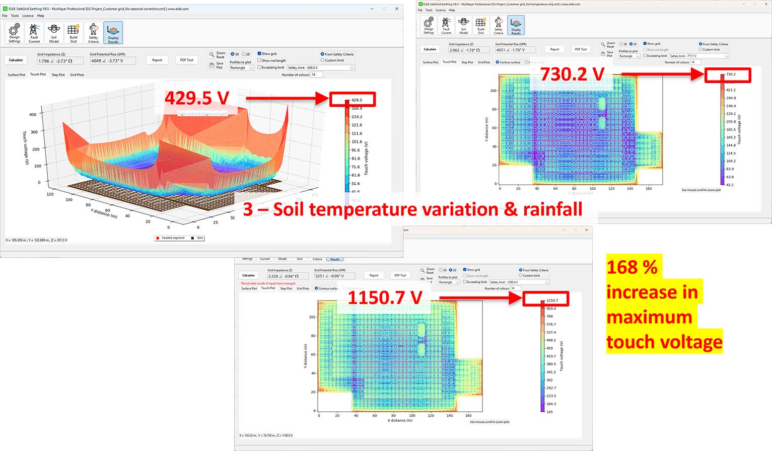
Soil resistivity varies throughout the year with soil temperature and moisture, and the change is greatest in the shallow layers that govern touch voltage. At a 132 kV substation in Sydney, correcting a March soil model to the worst day of the year raised the maximum touch voltage from 429.5 V to 1150.7 V, an increase of 168%. Unless measurements happened to fall on the worst day, an uncorrected soil model produces a non-conservative earthing design.
Why the worst day of the year governs earthing safety
Earthing design starts with a soil resistivity measurement, usually a Wenner four-point traverse taken in a single day. That measurement is then interpreted into a multilayer soil model and used to calculate earth grid resistance, grid potential rise and touch and step voltages for the design life of the installation.
The problem is that soil resistivity is not a fixed property. Electrical conduction through soil is largely electrolytic, so resistivity falls as temperature rises and falls as moisture content rises. Both quantities swing through an annual cycle, and both swing hardest in the top metre or two of soil. Touch voltage near an earth grid depends mainly on the resistivity of those shallow layers, so a soil model measured in mild, wet conditions can understate the touch voltage that will occur in cold or dry conditions by a factor of four.
This article covers the theory behind the effects of temperature and moisture on soil resistivity, a parametric study of four climate cases, and a real-world design for a 132 kV substation in Sydney, Australia. The modelling was performed using ELEK SafeGrid Earthing Software, which calculates multilayer soil models from field measurements, predicts the worst day of the year, and applies the resulting correction to the soil model before the earthing calculation is run.
How soil temperature and moisture change resistivity
Shallow layers govern touch voltage
Before looking at seasonal effects, it is worth establishing why the top of the soil profile matters so much. Earth grid resistance is determined primarily by the deeper layers, as current spreads far from the grid before dissipating. Touch voltage is set mainly by the topsoil, because it depends on the potential difference over a short distance at the surface.
Table 1: Effect of the soil model on grid resistance and touch voltage for the same earth grid.
| Soil model (top / bottom) | Resistance (Ω) | Grid potential rise (V) | Maximum touch voltage (V) |
|---|---|---|---|
| 100 / 1000 Ω·m | 12.104 | 12 104 | 1042.4 |
| 500 / 1000 Ω·m | 19.189 | 19 189 | 3572.9 (+243%) |
| 1000 / 100 Ω·m | 3.035 | 3035 | 1387.1 |
| 2000 / 100 Ω·m | 3.159 | 3159 | 1513.1 (+9%) |
Raising the top layer from 100 to 500 Ω·m increases touch voltage by 243%. Raising the bottom layer from 1000 to 2000 Ω·m, a change twice as large in absolute terms, increases it by only 9%. Any process that changes shallow resistivity, therefore, deserves attention.
Soil temperature
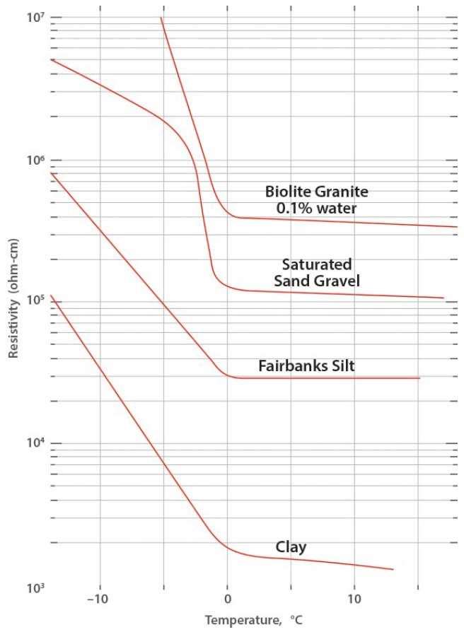
Lower temperatures reduce electrolytic activity and raise resistivity. The relationship divides into two distinct segments, either side of the freezing point, which usually sits slightly below 0 °C:
- Above freezing, the effect is moderate. A temperature rise of about 20 °C reduces resistivity by roughly 50%.
- Below freezing, the effect is severe. At about -10 °C, resistivity is 400% to 1000% higher than immediately before freezing because the pore water freezes, and ice is a very poor conductor.
Soil temperature with depth/lat
Soil temperature follows air temperature, but with attenuation and delay that both increase with depth. The ground surface is a balanced heat-transfer system of conduction, convection, thermal radiation, and evaporation, and the soil beneath it behaves as a damped, phase-shifted low-pass filter driven by the annual air temperature cycle.
The standard analytical form is a sinusoidal air temperature driving the diffusion equation in a semi-infinite medium:
\(T(z,t) = T_{m} + A \cdot exp\left(-z\sqrt{\frac{\pi}{\alpha P}}\right) \cdot sin\left[\frac{2\pi(t-t_{0})}{P} – z\sqrt{\frac{\pi}{\alpha P}}\right]\)
where Tm is the mean annual soil temperature, A is the amplitude of the annual air temperature swing, z is depth, α is the thermal diffusivity of the soil, P is the one-year period, and t0 relates the phase to the first day of spring. The exponential term attenuates the swing with depth, and the second phase term delays it. Soils with higher thermal diffusivity conduct temperature changes more readily.
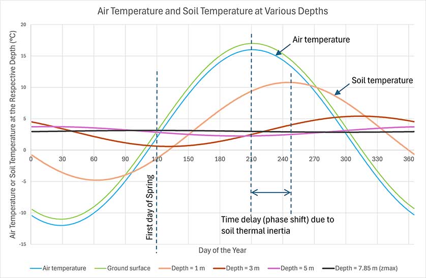
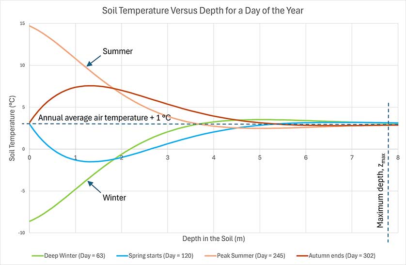
Figure 3 shows why the calendar alone is a poor guide. On the first day of spring, the soil is still colder than the air, because it retains the winter that has just ended. The worst day for soil resistivity is not the day of the lowest air temperature.
Soil moisture
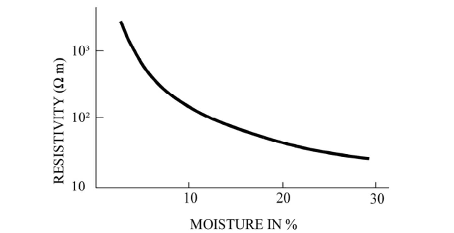
Resistivity also depends strongly on water content, and this dependence is steepest at low moisture levels. Water content influences soil resistivity strongly up to about 20%; above that, further wetting changes little.
Soil moisture varies with rainfall, snowmelt, diffusion, evapotranspiration, surface runoff and deep percolation. The practical modelling approach is a monthly water balance over an active soil layer, in which infiltration adds moisture in proportion to net rainfall and a loss term removes it. Because the annual rainfall pattern repeats, the moisture solution converges to a periodic steady state over the twelve months of the year, and that steady state is what the correction uses.
The effect of rainfall on moisture reduces with depth and effectively ceases below a critical depth of about 1 m. The moisture-based correction factor is therefore applied in full at the surface and blended linearly to unity at that critical depth.
Combining the two effects
The two mechanisms are treated as independent correction factors on the measured resistivity, each evaluated as a ratio between the measurement day and the calculation day, and each varying with depth:
\(k_{total}(z) = k_{temperature}(z) \cdot k_{moisture}(z)\)
The corrected soil model is the measured model multiplied layer by layer by k_total. Because both factors approach unity with depth, correction subdivides and modifies the shallow layers while leaving the deep layers unchanged. This is why a corrected model typically has more layers than the measured one.
Parametric study: four climate cases
To separate the effect of temperature from the combined effect of temperature and moisture, the same measured soil model was corrected under four conditions on a 20 m by 20 m square earth grid with rods. The measured model in every case is 23.34 Ω·m over 1.53 m, then 47.88 Ω·m over 39.94 m, over 183.02 Ω·m. Soil type is clay.
Table 2: Parameters for the four climate cases.
| Case | Climate | Effects included | Mean annual ground temperature | Annual air temperature fluctuation | Measurement day | Worst day |
|---|---|---|---|---|---|---|
| 1 | Hot to moderate, southern hemisphere | Temperature | 19.45 °C | 3.16 °C | 5 February | 8 August |
| 2 | Hot to moderate, southern hemisphere | Temperature and rainfall | 19.45 °C | 3.16 °C | 30 November | 31 July |
| 3 | Cold, northern hemisphere | Temperature | 3.14 °C | 17.81 °C | 24 July | 23 January |
| 4 | Cold, northern hemisphere | Temperature, rainfall and snowfall | 3.14 °C | 17.81 °C | Recalculated with precipitation included | Recalculated with precipitation included |
Adding rainfall to case 1 shifts both the measurement day and the worst day, because the day with the minimum average resistivity is no longer determined solely by temperature.
Table 3: Corrected top layer resistivity and maximum touch voltage for each case. The uncorrected model gives 280 V.
| Case | Top layer resistivity on the worst day (Ω·m) | Maximum touch voltage (V) | Increase |
|---|---|---|---|
| Uncorrected | 23.34 | 280 | - |
| 1: hot, temperature | 28.33 | 313 | 11% |
| 2: hot, temperature and rainfall | 82.58 | 1158 | 313% |
| 3: cold, temperature | 2214.4 | 373 | 33% |
| 4: cold, temperature and precipitation | 5036 | 1171 | 317% |
Two results stand out. First, in a hot climate, the temperature effect alone is modest, an 11% rise in touch voltage, because the annual air temperature swing is small and the soil never approaches freezing. Second, moisture is the dominant mechanism in both climates. Adding rainfall takes the hot case from 11% to 313%, and adding precipitation takes the cold case from 33% to 317%. A seasonal correction that considers temperature only will miss most of the effect.
Case 4 also shows why the two mechanisms compound rather than cancel. Soil temperature in the shallow layers is close to in phase with air temperature, and at this location, the moisture cycle is roughly in phase with it as well. Cold and dry arrive together, and both push resistivity in the same way.
Case study: 132 kV substation earthing design in Sydney
A 132 kV substation is being installed in Sydney, Australia. Soil resistivity measurements were taken on 15 March 2024. The design question is what the touch voltages will be on the worst day of the year, rather than on the day of measurement.
Parameters for modelling
| Input | Value | Source |
|---|---|---|
| Measurement date | 15 March 2024 | Wenner four-point traverse |
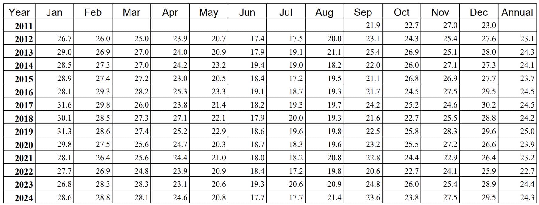
| Mean annual air temperature | 22.7 °C | Bureau of Meteorology, minimum of all available years |
| Mean annual soil temperature | 23.7 °C | Air temperature plus 1 °C |
| Annual air temperature fluctuation | 23.6 °C | 22.7 °C minus -0.9 °C |
| First day of spring | 1 October | The day when the mean daily temperature equals the mean annual temperature |
| Monthly rainfall | Monthly mean for all years | Bureau of Meteorology |
| Soil type for thermal properties | Silt | Geotechnical report |
Three inputs deserve comment.
Choosing conservative weather data. The minimum value across all available years was used for the mean annual air temperature, rather than the average across all years, because soil resistivity is higher at lower temperatures. The same logic sets the annual fluctuation from the extreme values rather than the typical ones.
Choosing the soil type. The geotechnical report gives silt from the surface to 0.3 m, clay from 0.3 m to 1.9 m, and clayey sand from 1.9 m to 3 m. Silt was selected because it is the topsoil layer and has higher thermal diffusivity than clay, so it transmits temperature changes more deeply. A single soil type is assumed to represent the thermal and moisture behaviour of all shallow layers, which is reasonable because temperature and moisture variations affect only the shallow layers.
Defining the first day of spring. This is the day in early spring when the average daily temperature equals the average annual temperature, which for this site is 1 October. It sets the phase of the soil temperature solution, so an error here shifts the predicted worst day.
Predicting the worst day and the corrected soil model
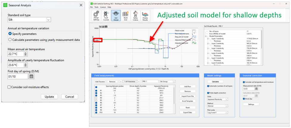
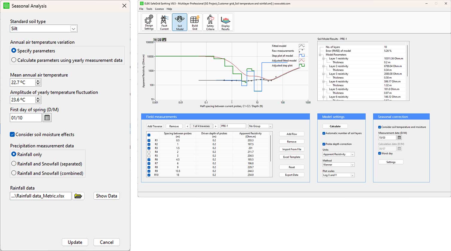
With temperature effects only, the worst day is 5 July. With temperature and moisture combined, the worst day moves to 30 July. In both cases, the correction subdivides the shallow layers of the measured model and raises their resistivity, leaving the deeper layers unchanged.
Touch voltage results
| Soil model | Maximum touch voltage (V) | Increase compared with the uncorrected case |
|---|---|---|
| Uncorrected, measured 15 March | 429.5 | - |
| Corrected for soil temperature, worst day 5 July | 730.2 | 70% |
| Corrected for soil temperature and rainfall, worst day 30 July | 1150.7 | 168% |
| Soil model | Maximum touch voltage (V) | Increase compared with the uncorrected case |
|---|---|---|
| Uncorrected, measured 15 March | 85.2 | - |
| Corrected for soil temperature | 157.6 | 85% |
| Corrected for soil temperature and rainfall | 365.3 | 328% |
The larger grid has lower absolute touch voltages because it equalises the surface potential more effectively, but it has a higher proportional sensitivity to shallow resistivity. A design that passes comfortably on the measured model can fail on the corrected one.
Validation
The temperature model was checked against a published field campaign in which vertical electrical soundings were repeated monthly for a year at a single site in a temperate coastal climate, giving twelve measured apparent resistivity profiles over the annual cycle.
Using March sounding as the measurement day and predicting the June profile, the temperature-only correction yields a 16% increase in top-layer resistivity. The measured apparent resistivity at 0.5 m probe spacing increased by 108% over the same period. The direction and the timing are right, but the magnitude is short by a wide margin.
That gap is what the moisture model closes. Rainfall at the site is far higher in March than in June, so the top layer is much wetter on the measurement day than on the calculation day. When the moisture correction is included, the apparent resistivity computed from the corrected model agrees more closely with the measured sounding, particularly at the small probe spacings that resolve the shallow layers. The same improvement appears when the measurement and calculation days are swapped, which confirms the correction is symmetric rather than tuned to one direction.
This validation is also the clearest practical argument for not stopping at temperature. In a temperate coastal climate, the temperature-only correction captured less than a fifth of the measured change.
Practical design procedure
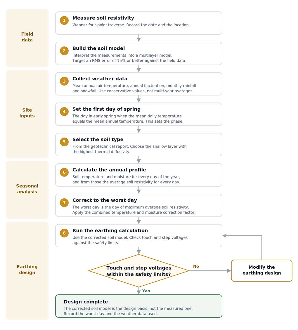
- Always take soil resistivity measurements (do not guess) and record the date. Without the date, the correction cannot be calculated, because it is a ratio of the measurement day to the worst day.
- Interpret the measurements into a multilayer soil model. An RMS error of 15% or better against the field data is a reasonable target.
- Obtain weather data for the site: mean annual air temperature, annual air temperature fluctuation, and mean monthly rainfall and snowfall. Use the minimum mean annual temperature and the maximum fluctuation on record, not the multi-year average.
- Determine the first day of spring, the day in early spring when the mean daily temperature equals the mean annual temperature. This sets the phase of the soil temperature solution, so an error here shifts the predicted worst day.
- Select the soil type from the geotechnical report. Where several soils appear in the shallow layers, choose the one with the highest thermal diffusivity, because it carries the temperature swing deeper and gives the more onerous correction.
- Calculate soil temperature and moisture for every day of the year, and from those, the average soil resistivity for every day.
- Identify the worst day, the day of maximum average soil resistivity, and apply the combined correction factor to the measured soil model. The worst day is defined by the depth-averaged resistivity, so it will not always coincide with the exact day of maximum touch voltage.
- Run the earthing calculation on the corrected model and check touch and step voltages against the safety limits.
- If the design does not comply, modify the earthing design and repeat step 8. Do not revert to the measured soil model. Record the worst day and the weather data used, so a reviewer can reproduce the result.
Key engineering takeaways
- Touch voltage is governed by the resistivity of shallow soil. Raising the top layer from 100 to 500 Ω·m increased touch voltage by 243%, while doubling the bottom layer changed it by 9%.
- It is unlikely that measurements were taken on the worst day of the year. Check this rather than assume it. The worst day for the Sydney site was 30 July, more than four months after the March measurement.
- Correct for moisture and temperature. Temperature alone accounted for an 11% increase in touch voltage in the hot-climate case, compared with 313% when rainfall was included.
- Seasonal correction matters in hot climates, too. It is not only a frozen ground problem. The Sydney case gained 168% on a site that never freezes.
- Apply the correction to depths of about 10 m. Below that, temperature and moisture variations are negligible, and the measured model stands.
- Use conservative weather inputs. Take the minimum mean annual temperature and the maximum fluctuation from the available record, not the multi-year average.
- Larger grids are proportionally more sensitive. The 300 m by 300 m grid achieved 328%, compared with 168% for the smaller grid on the same site.
- Choose the shallow soil type with the higher thermal diffusivity when the geotechnical profile has several. Higher diffusivity carries the temperature swing deeper and gives a more onerous result.
FAQ
When should I apply a seasonal correction to soil resistivity measurements?
Every time, unless you can demonstrate that the traverse fell on the worst day of the year. You need three things, all of which are easy to get: the test date, the site location, and monthly temperature and rainfall normals from the National Weather Service. If you have those, there is no reason to skip it.
What if nobody recorded the date of the soil resistivity test?
Then you cannot correct it because the correction is a ratio of the measurement day to the worst day. Your options are to remeasure with the recorded date or to assume the measurement landed on the best day of the year and correct from there, which is the conservative bound. This is the strongest practical reason to write the date on the test sheet.
Does this matter if the ground never freezes?
Yes. Freezing yields the largest jump in resistivity, and the cold-climate case here shows a 313% increase attributable solely to temperature. But the Sydney site never approaches freezing, and correcting for temperature and rainfall still raised the maximum touch voltage by 168%. Where soil does not freeze, moisture is the mechanism that matters.
Can I just measure again in winter and skip the analysis?
A second set of measurements is worth having, but it does not replace the correction. A winter traverse reduces the size of the correction; it does not remove the need to calculate it, and it does not tell you how close you got. At the Sydney site, the worst day was 5 July for temperature alone and 30 July once moisture was included, so even a winter measurement can miss by weeks. The better use of a second set is as a check: correct both to the same worst day and see whether the two corrected models agree.
Does the correction change the grid resistance and the grid potential rise, or only the touch voltage?
Both move, by very different amounts. For the 300 m grid at the Sydney site, the grid potential rise increased from 1129 V to 1549 V, about 37%, while the maximum touch voltage increased by 328 V. Grid resistance is set by the deeper soil, which the correction barely reaches. Touch voltage is set by the top metre or two, which is where the entire correction lands.
Does a crushed rock surface layer protect me from this?
Not in the way most people assume. Where the surface is bare soil, correcting the model raises both the calculated and permissible touch voltages, and the two partly cancel. Where the site is surfaced with wet crushed rock at 3000 Ω·m, the permissible voltage is fixed by the rock, so the full increase in touch voltage comes straight out of your margin.
How deep does the correction reach?
The temperature reaches about 10 m. Moisture is far shallower because rainfall no longer changes soil moisture below roughly 1 m, so the moisture factor is applied in full at the surface and blended to unity at that depth. Below about 10 m, the measured model stands unchanged.
Why does the worst day move once rainfall is included?
With temperature alone, the worst day occurs near the annual temperature minimum, pushed later by the soil’s thermal lag. Rainfall has its own annual cycle with a different phase, so combining the two shifts where the maximum falls. In the hot-climate example, the worst day moved from 8 August to 31 July, and at the Sydney site, it moved from 5 July to 30 July.
The geotechnical report identifies three soil types in the top few metres. Which one do I use?
The shallow one with the highest thermal diffusivity. At the Sydney site, the silt was in the top 0.3 m, not the clay below it. Higher diffusivity carries the annual temperature swing deeper, so it produces a more onerous correction. The analysis assumes that a single soil type represents all the shallow layers, which is acceptable because only those layers move.
References
[1] IEEE Std 80-2013. IEEE Guide for Safety in AC Substation Grounding.
[2] IEEE Std 81-2012. IEEE Guide for Measuring Earth Resistivity, Ground Impedance, and Earth Surface Potentials of a Grounding System.
[3] IEEE Std 142-2007. IEEE Recommended Practice for Grounding of Industrial and Commercial Power Systems (IEEE Green Book).
[4] IEC 61936-1:2021. Power installations exceeding 1 kV AC and 1.5 kV DC. Part 1: AC.
[5] EN 50522:2022. Earthing of power installations exceeding 1 kV AC.
[6] AS 2067:2016. Substations and high voltage installations exceeding 1 kV AC.