Table of Contents
Overview: Testing of earth grid performance
Testing of earthing system performance plays a vital role in ensuring safe power systems operation. The fall of potential (FOP) method is common for performing impedance tests, especially for large and complex earthing grids. While the FOP method is useful, it has its limitations and using software simulations can greatly improve how engineers approach these tests.
By using software models, engineers can determine the best way to set up grid impedance tests and better predict how they will turn out. This helps validate important soil and earthing system models used during the design phases. This technical article dives into how software simulations make grid impedance tests more accurate, helping to improve electrical earthing system design and performance.
ELEK SafeGrid Earthing Software has been used for the modelling.
Why measure earth grid resistance
Although the measured impedance of an earthing system is often referred to as resistance, there is a reactive component that can be of significant magnitude for large or interconnected grids.
The important reasons why we measure earthing system impedance include [1]:
- To verify the performance of a newly installed earthing system. Normally the calculated value determined during the design phase is compared with the measured value.
- To detect changes in an existing grounding system. A significant variation in a measured value between periods may indicate severe deterioration or another situation of concern.
- To determine grid potential rise (GPR) for the design of protection for power and communication circuits.
The main methods for measuring earthing system impedance (in order of setup complexity and accuracy) include the two-point method, the three-point method, and the four-point commonly known as the fall of potential (FOP) method.
It’s relatively easy to measure the impedance of small earthing systems compared with large ones. The FOP method is preferred for measuring the impedance of large earthing systems. The main advantage of the FOP method is the voltage, and current electrodes can have a substantially higher resistance than the grid being tested without significantly affecting the accuracy of the measurement.
The Fall of Potential Test explained
With the FOP test method, the resistance of an earthing system is measured using a remote earth electrode. An alternating current (AC) source is connected to the grid being measured to measure grid resistance, and the remote earth electrode causes a current to flow through the soil. A voltage measurement circuit is then connected to the main earthing system, and a sensitive voltage measurement device is used to measure the ground surface voltage at points equidistance apart along a line starting from the earthing system toward the remote electrode. Figure 1 shows the test setup for an earth grid using the FOP method.

The measured surface voltages are converted into apparent impedance as follows:
Apparent resistance = (grid injection point voltage – surface point voltage of voltage electrode) / injected current.
For a given current electrode location, there is one voltage electrode spacing that gives the true grid impedance of the earthing system being tested. There is a theoretical position of 61.8 % of the separation distance between the measured earth grid and the current electrode, which is the correct position for measuring the exact impedance for uniform soil resistivity (and numerous other assumptions).
Apparent impedance is plotted versus the voltage electrode distance X from the grid being measured Figure 2. The shape of the apparent impedance curve between the grid being measured and the remote electrode should rise steeply, flatten out (rise slowly) towards the middle, representing a zone where the interaction of the tested and return electrodes is small, and (for zero-degree tests) rise again steeply approaching the remote electrode.

Important questions to answer about earth resistance tests
How far away from the grid should the current electrode be placed?
The remote electrode should ideally be located at an infinite distance from the earthing system where the earth’s current density approaches zero. The remote electrode is located at a distance of at least five (5) times the maximum diameter of the measured earthing system [1].
Locating the current and the voltage electrodes approximately 6.5 times the extent of the earthing system will measure 95% of the earthing impedance. Extended to 50 times the maximum earthing system dimensions will give an expected measurement accuracy of only 98.5% [2].
Once the criteria for the current electrode are satisfied, the location of the voltage electrode needs to be away from the influence of the grid under test and the current electrode to accurately measure the earthing impedance.
What direction and how far should the voltage electrode be run?
Earthing impedance can be estimated by moving the voltage electrode between the grid under test and current electrode location (0° test). This direction is often the most convenient since current leads are already run there. There are two ways of estimating the measured impedance:
- The impedance is theoretically obtained at a voltage electrode distance, which is 61.8 % of the separation distance between the measured earth grid injection point and the remote current electrode; or
- If two or three consecutive measurements provide a constant value, then the voltage electrode is out of the influence of the other electrodes, and the measurement is assumed to represent the true impedance value (flat slope method).
Serious problems exist for these methods including that the assumptions of the 61.8 % rule are often violated and often for multilayered soils no flat slope exists.
For voltage measurements in the opposite direction (180° test) to the current electrode, the dashed line shown in Figure 2 will always be approaching the solid line from below, and the required separation distance is much greater which can be a problem (theoretically 161.8 % of the separation distance between the grid and current electrode – see Annex C of [1] for the derivation). A further problem is the results have increased sensitivity to soil non-uniformity [1].
It is recommended to perform voltage measurements at a right angle (90° test) for testing low impedance earthing systems of 1 Ω or less [1]. This avoids introducing significant errors to the measurements caused by AC mutual coupling between the test leads of the current and voltage electrodes. Often it is impossible or impractical to measure at exactly 90° and this will introduce errors in the measured voltages. For an angle less than 90°, any voltage produced in the voltage lead, due to the coupling from current flowing in the current lead, is additive to the desired measured voltage. With angles greater than 90°, the opposite effect exists; the mutually coupled voltage is negative and results in a reduction in the measured impedance.
Because the mutual coupling is less in magnitude, orientations of 90–180° and 180–270° are preferred over those of 0–90° and 270–360° [2].
What are the limitations of the earthing resistance test?
The limitations of the FOP testing method include:
- An accurate measurement of apparent impedance is possible only when the grid’s current density fields produce a hemisphere with an electrical centre. It may be very difficult to obtain a result for grids that are either large or complex in shape or with interconnected earth return paths.
- The 61.8 % rule does not apply for non-homogeneous (multilayered) soils, and the apparent resistance curve’s flat portion may lie between 10 % and 90 % along the distance.
In non-homogeneous soils, the appropriate probe position cannot be determined by simple observation of the shape of the apparent resistance curve. Rather, a computer simulation of the grounding system and test circuit must be performed to predict the appropriate voltage probe position [3].
Software modelling
Software modelling of a FOP test for an earthing system can be useful for the following reasons:
- To establish the optimal test setup, such as determining the required minimum current electrode separation from the main earthing system, prior to testing.
- To check the validity of soil resistivity and earthing system models used during the design phase.
For an accurate comparison between the measurements and calculated values, the grid impedance test should occur without the connection of overhead earth wires, or with other earthing systems providing alternative fault current pathways. For new earthing systems, this occurs just after construction.
The impedance of a new earth grid will usually decrease slightly as the disturbed earth settles to its natural compactness, a year or more after construction [1].
How to model an earth grid resistance test?
The grid under study and the remote electrode are modelled, and a unity current is simulated as flowing between them. Ground surface voltage is measured along a line in the simulation, just like in the test. The complete step-by-step procedure is explained in the Simulate a Fall of Potential Test tutorial [ref. 4].
Case study - Substation earth grid resistance
The earth grid is 60 by 30 metres with 28 off vertical rods, as shown in Figure 3. The soil model is three-layered with a top layer 100 Ωm of 1 m thickness, middle layer 200 Ωm of 1 m thickness, and bottom layer 300 Ωm of infinite thickness. A remote current electrode was added to the model and located at five times greater than the maximum diagonal of the primary grid. In this case, the diagonal distance of the grid is approximately 67 m; therefore, the remote current electrode is located at x = 390 m.
")
According to the Fall of Potential rule, the calculated grid impedance is expected to be at a distance of 61.8 % from the current injection point. In our case 222 m is 61.8 % away from the injection point. Zooming into the touch plot at 222 m, we can see that the apparent impedance at that point is 2.5 Ω which corresponds to the apparent grid impedance calculated in SafeGrid.
Closer examination of the difference between the theoretical 61.8 % and the accurately calculated SafeGrid impedance value reveals a small error of 0.41 %.

")
Case study – Effect of coupling between voltmeter and current generator leads
In this case study, we consider a 100 m by 100 m 16-mesh grid buried in uniform soil with a low resistivity value of 10 Ωm at a depth of 0.5 m. The exact grid impedance at 80 Hz from a 0.5 m rod that connects the grid center to the earth’s surface is 0.052 Ω (angle of 6.07 degrees). The distance of the FOP return current electrode from the grid injection point on the ground is 1000 m, which is more than 5 times the grid diagonal. We also considered insulated leads for the current generator and the voltmeter used in the zero-degree-FOP tests. We assumed that the locations of the voltmeter and current generator, as well as their wire leads, are 1 m apart. The spacing between the voltmeter input terminals is 1 cm, and so is the spacing between the current output terminals of the generator. The following diagram shows the apparent resistivity of the zero-degree FOP tests versus voltage electrode distance X. The FOP results with no wire leads are also included for comparison purposes. With no leads, we observe that the curve exhibits a wide flat zone in which the FOP apparent impedance is very close to the actual grid impedance. When the leads are present, the resulting FOP impedance magnitude and angle values are very far from the actual grid impedance value.
 Vs Voltage probe distance from grid")
 Vs Voltage probe distance from grid")
The large error is due to the long lead wires for the current injection and voltmeter, which are only 1 m apart. If the spacing between the leads is increased, the error is reduced to some extent in zero-degree FOP tests [6]. An effective way to mitigate the lead effect is to apply alternative FOP methods, such as 90-degree FOP. The following figure shows the results associated with 90-degree tests on the same grid, the same current loop spacing, and the same frequency as before, with and without the leads. We also applied the same voltage probe distance values as before but in a perpendicular direction. In the 90-degree test without the leads, we observe that apparent impedance approaches the exact grid impedance in both magnitude and angles when the voltage probe distance from the grid injection point is about half of the current loop spacing or more. Our examinations indicate that this minimum distance is reduced with frequency increase (results not shown here). The results obtained with the leads for apparent impedance magnitude indicate minor differences compared to those with no leads. The differences in the impedance angles due to the lead effect are larger than those of the magnitude but compared to the zero-degree FOP, they are much smaller and follow similar trends. This improvement compared to zero-degree FOP is due to the fact that the voltage leads follow a path that departs away from the current leads as the voltage probe distance is increased.
 Vs Voltage probe distance from grid")
 Vs Voltage probe distance from grid")
Recommendations for earthing resistance testing
The fall of potential (FOP) method is common for performing impedance tests, especially for large and complex earthing grids. Here are some suggestions for the testing setup:
- Extend the current electrode out to at least 5 times the diagonal dimensions of the grid.
- For grids with impedance of 1 Ω or less, perform voltage measurements at a right angle (90°) to the current electrode. If exactly 90° can’t be achieved, ensure it’s between 90° and 180°.
- Large measurement errors occur when long voltage measurement leads run parallel to current injection leads, particularly in low-resistivity soils. To mitigate this, it’s recommended to measure at a 90° angle.
- The grid impedance test should occur without the connection of overhead earth wires, or with other earthing systems providing alternative fault current pathways.
- Model the fall of potential test setup using software, prior to performing the tests.
To accurately determine the earth grid impedance, we make the following recommendations:
- The fall of potential test will not give accurate results for very large, complicated, or odd-shaped grids.
- The 61.8 % rule will give reasonable results, even for multilayered soils, unless the soil model is low on high resistivity.
- Model the fall of potential test results using software to validate the site measurements.
References
[1] IEEE Std 81-2012, IEEE Guide for Measuring Earth Resistivity, Ground Impedance, and Earth Surface Potentials of a Grounding System.
[2] IEEE Std 81.2-1991, IEEE Guide for Measurement of Impedance and Safety Characteristics of Large, Extended or Interconnected Grounding Systems.
[3] IEEE Std 80-2013, IEEE Guide for Safety in AC Substation Grounding.
[4] Simulate a Fall of Potential Test Tutorial, https://elek.com/tutorials/safegrid/how-to-simulate-a-fall-of-potential-test/
[5] ELEK SafeGrid Earthing Software, V8.0.