Table of Contents
A steady-state ampacity calculation assumes a cable carries its worst-case current continuously. Most circuits do not. Sized by the steady-state method, the 240 mm² aluminium feeder in this example rates ~290 A. Under its actual solar duty, peaking at 238 A for a few midday hours, the conductor settles near 50 °C, about 40 °C below the 90 °C XLPE limit. That margin below the limit means the cable can carry more current under this profile than the steady-state rating allows. This article covers how dynamic (cyclic) rating quantifies it, the applicable standards, and the modelling errors that invalidate it.
The example is an LV/MV PV collector. The method is voltage-independent: it applies equally to HV transmission and submarine export cables.
Steady-state vs dynamic rating
Cable current varies with load. The cable, duct, backfill and soil have thermal inertia, so conductor temperature lags the current and does not reach the steady-state value during short peaks. A steady-state rating (IEC 60287) assumes the peak current is continuous, at 100% load factor. A dynamic (cyclic) rating instead determines the current the cable can carry under the actual load profile while keeping the peak conductor temperature within its limit. Because the peak is brief, the current exceeds the steady-state rating; IEC 60853 expresses the increase as a cyclic rating factor applied to the steady-state value.
The results below were produced with ELEK Cable HV™ Software, whose transient thermal calculation is based on the IEC 60853 and CIGRE Electra No. 87 methods and is validated against the finite element method (IEC TR 62095 and CIGRE).
Worked example: five buried solar feeders
Five PV arrays each feed an inverter; each inverter supplies one buried feeder of three single-core 240 mm² aluminium XLPE cables (1.8/3 kV, operated at 800 V) in trefoil inside an air-filled 110 mm duct. The five feeders run side by side, 0.75 m above the duct, spaced 0.25 m apart, in native soil (1 K·m/W, ambient 20 °C). Conductor limit 90 °C.
Each feeder follows the solar profile: near zero overnight, a broad midday peak. At the ~290 A steady-state rating, a feeder carries ~400 kVA at 800 V; the 238 A peak is ~330 kVA of clear-sky output.
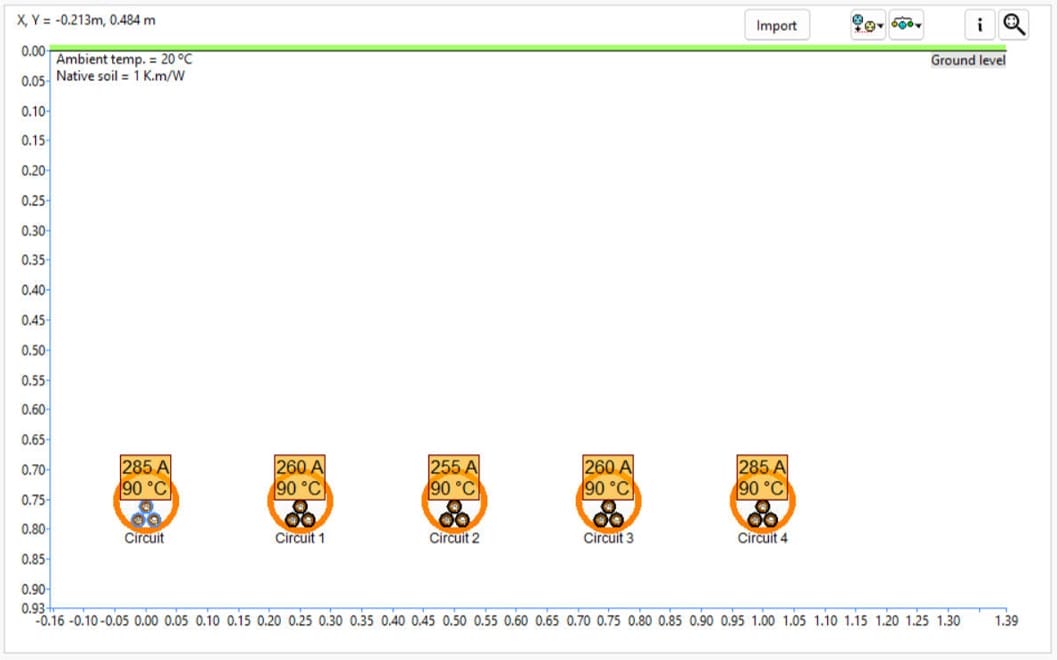
Table 1: Steady-state current rating per circuit (the centre circuit rates lowest, from mutual heating).
| Circuit | 1 | 2 | 3 | 4 | 5 |
|---|---|---|---|---|---|
| Steady-state current (A) | 285 | 260 | 255 | 260 | 285 |
The same 24-hour profile is applied to every circuit, peaking at 238 A in hours 11-14 and falling to ~10 A overnight.
Table 2: Daily load profile applied to every circuit (hourly load current, repeated every 24 hours).
| Hour | Load current (A) | Hour | Load current (A) |
|---|---|---|---|
| 1 | 11 | 13 | 238 |
| 2 | 11 | 14 | 238 |
| 3 | 11 | 15 | 227 |
| 4 | 11 | 16 | 187 |
| 5 | 14 | 17 | 135 |
| 6 | 33 | 18 | 78 |
| 7 | 89 | 19 | 26 |
| 8 | 145 | 20 | 13 |
| 9 | 197 | 21 | 10 |
| 10 | 233 | 22 | 10 |
| 11 | 238 | 23 | 10 |
| 12 | 238 | 24 | 10 |
Initial condition: preloaded vs no-load start
The transient result depends on the initial conductor temperature, so two bounding cases apply.
Preloaded start (conductor at the 90 °C limit). Each circuit is preconditioned to its maximum steady-state temperature, 90 °C, then the daily cycle is applied. Because the cyclic load is well below the preload current, the conductor cools, reaches a minimum overnight, and re-heats to a daily peak near hour 14. The cycle is repeated until the day-to-day change in peak temperature is < 0.1 °C:
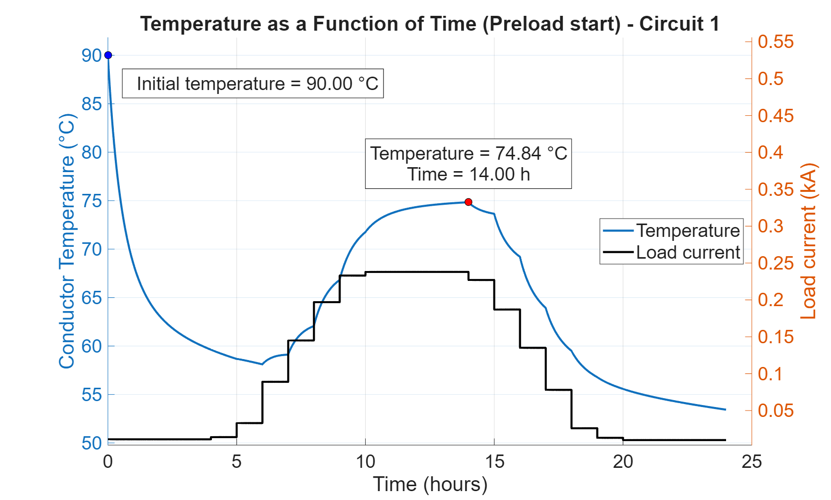

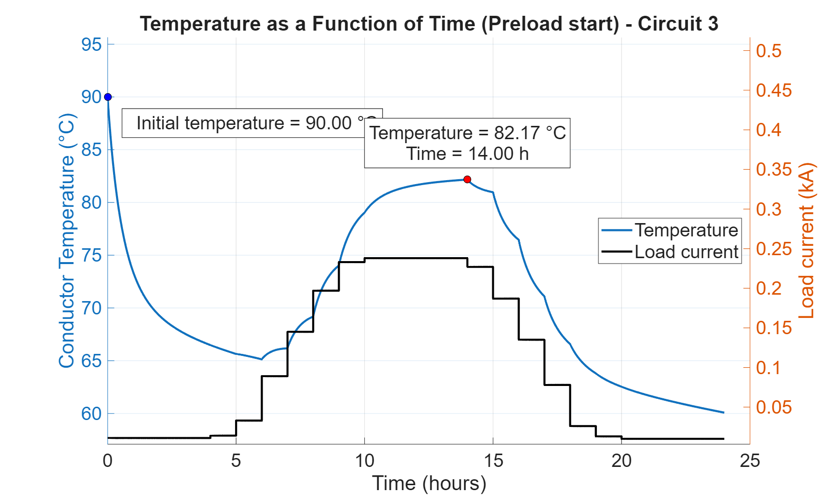
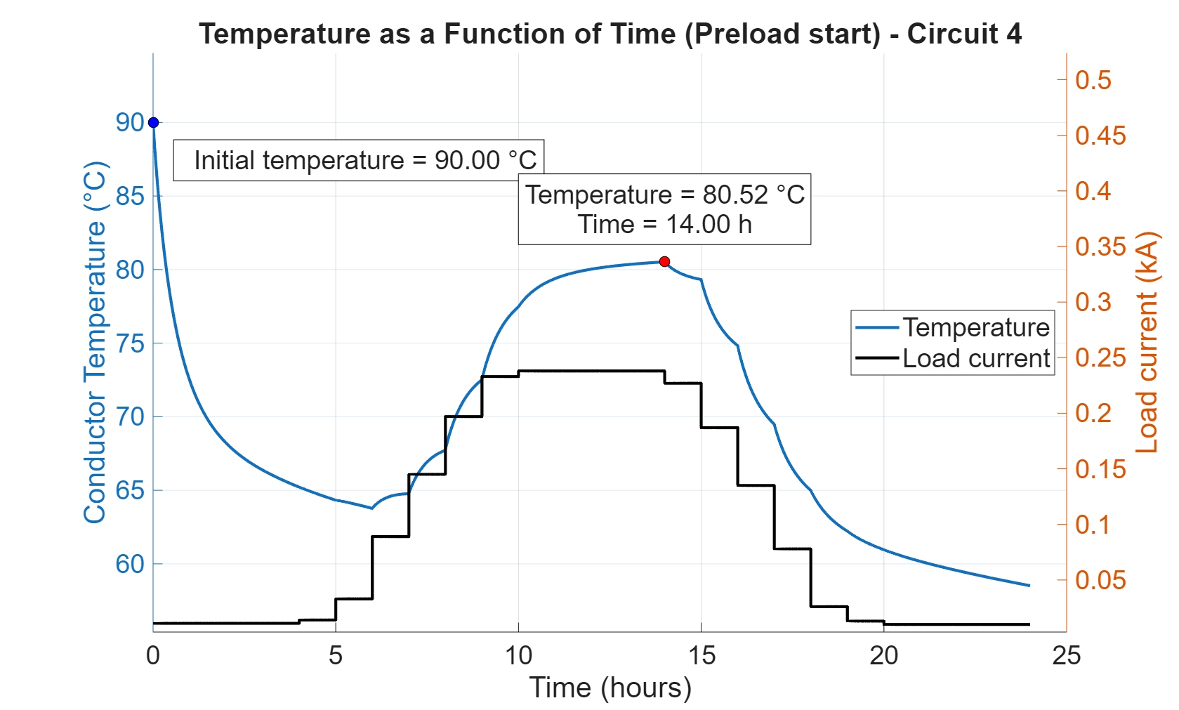
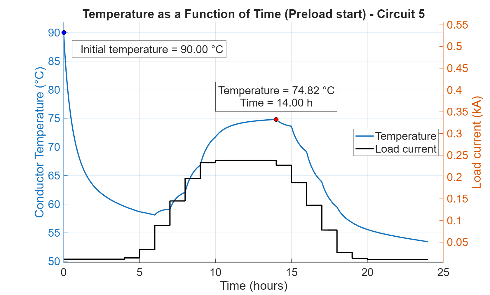
Figure 2 (a to e): Preloaded start. Conductor temperature and load current over 24 hours, circuits 1 to 5.
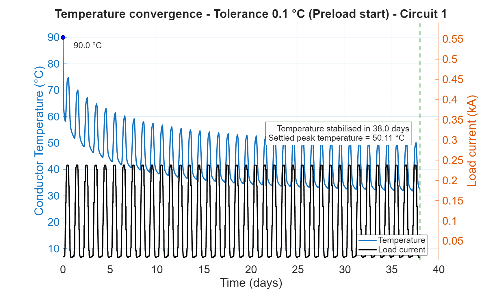
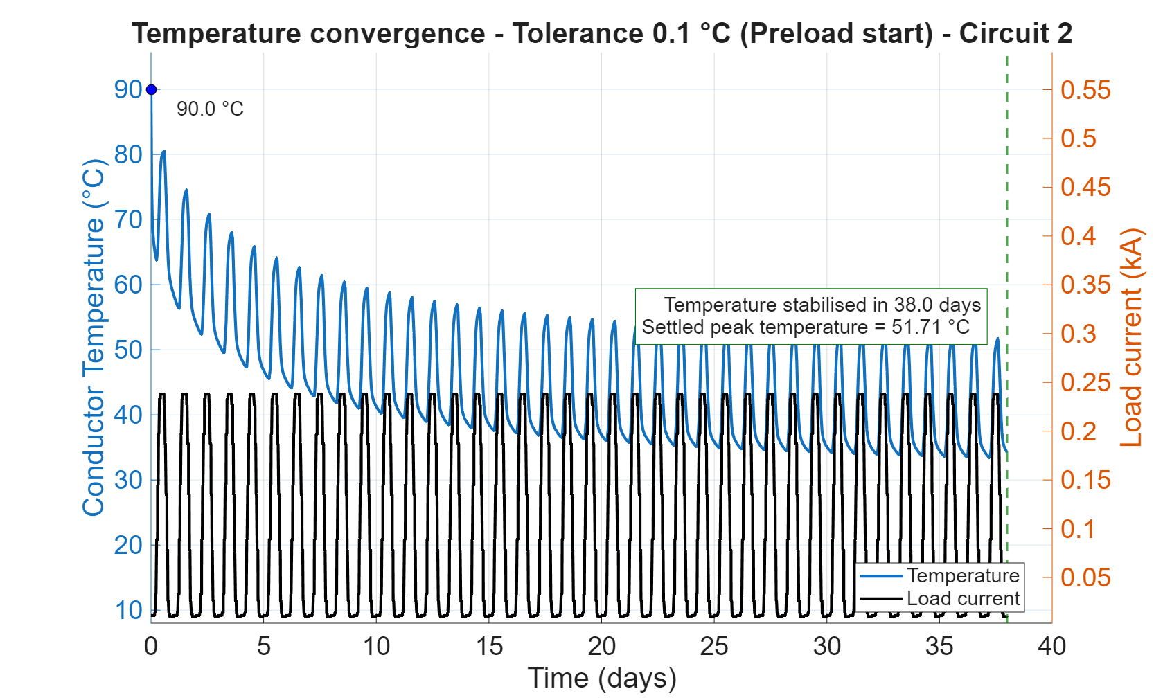
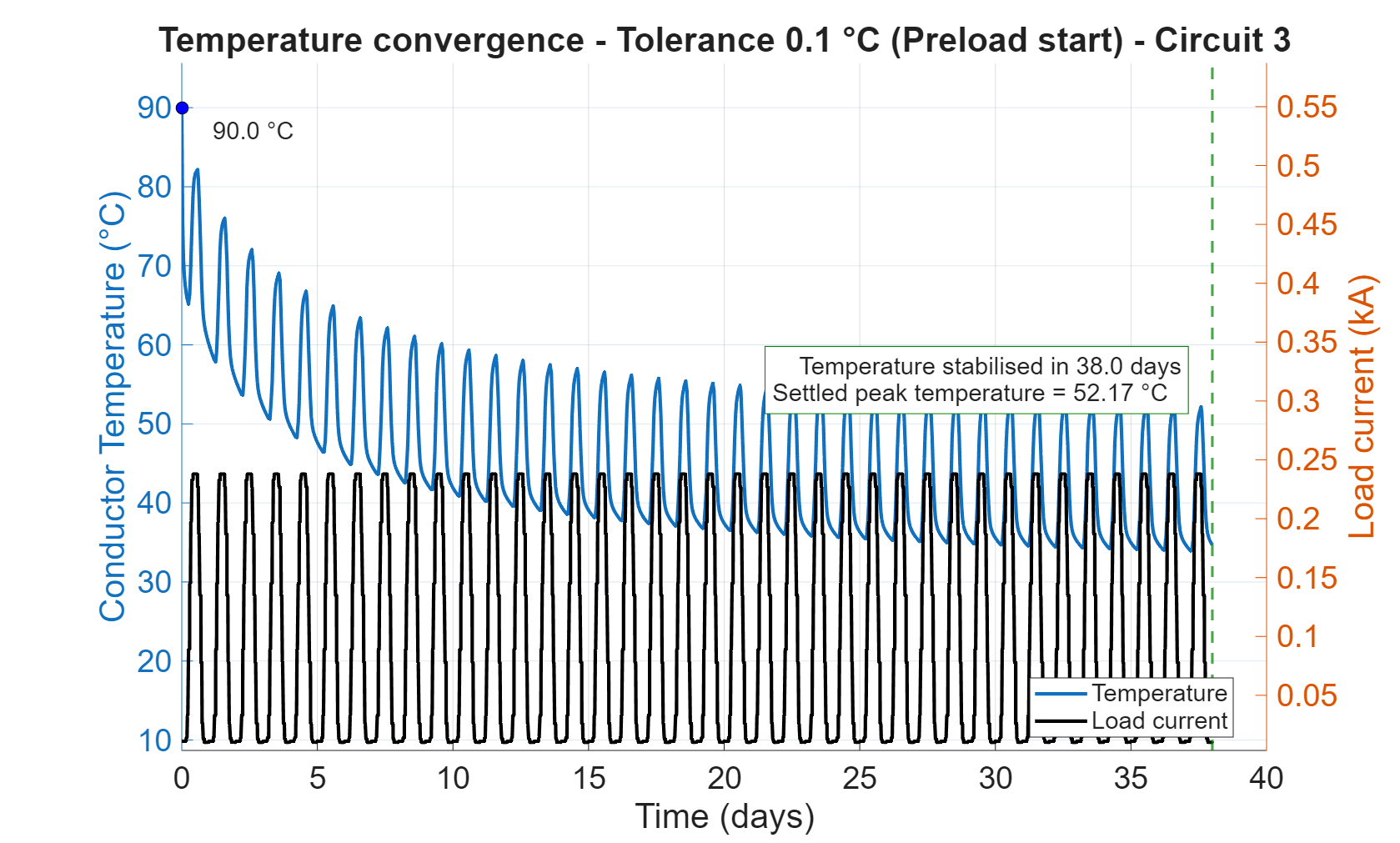


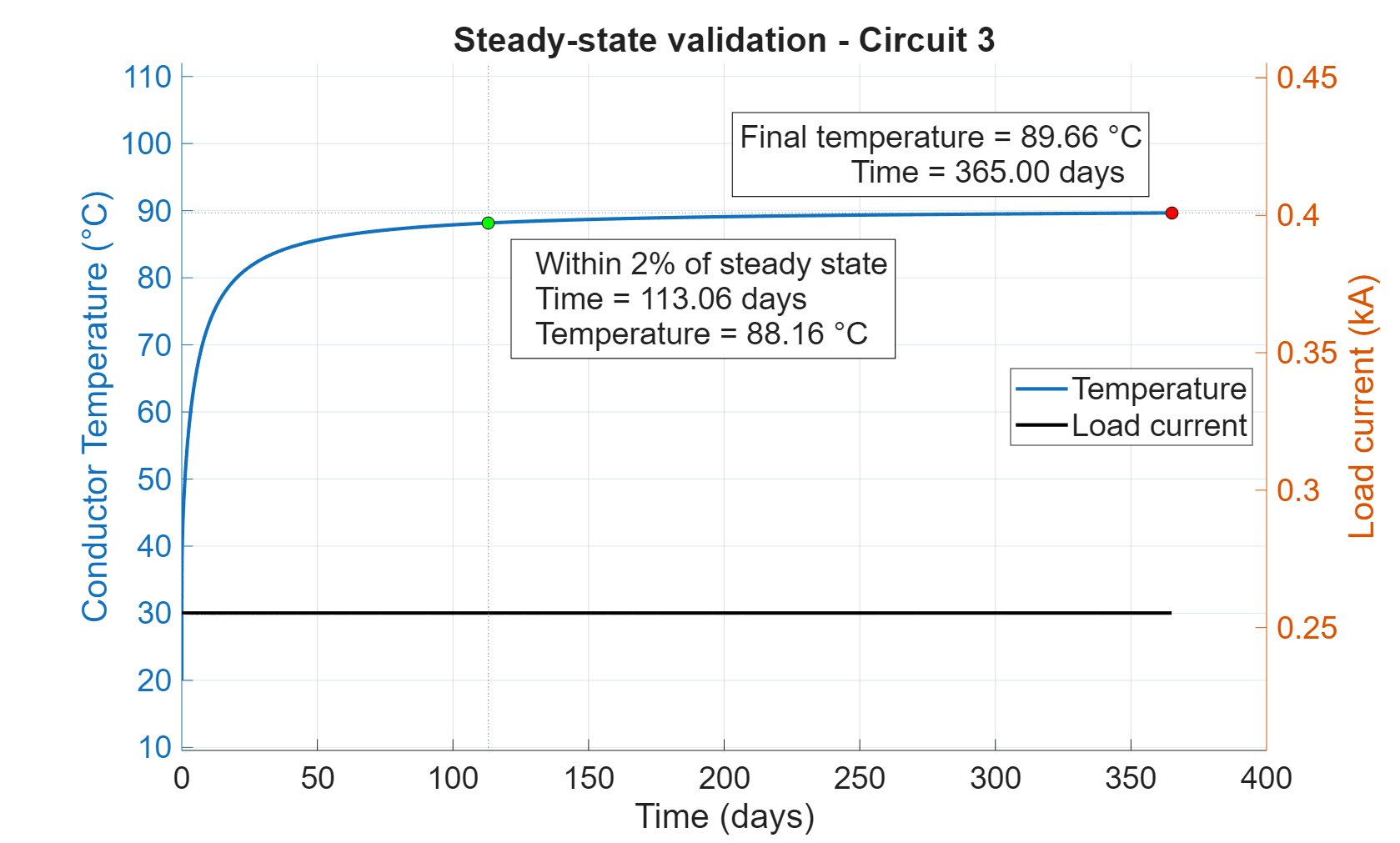
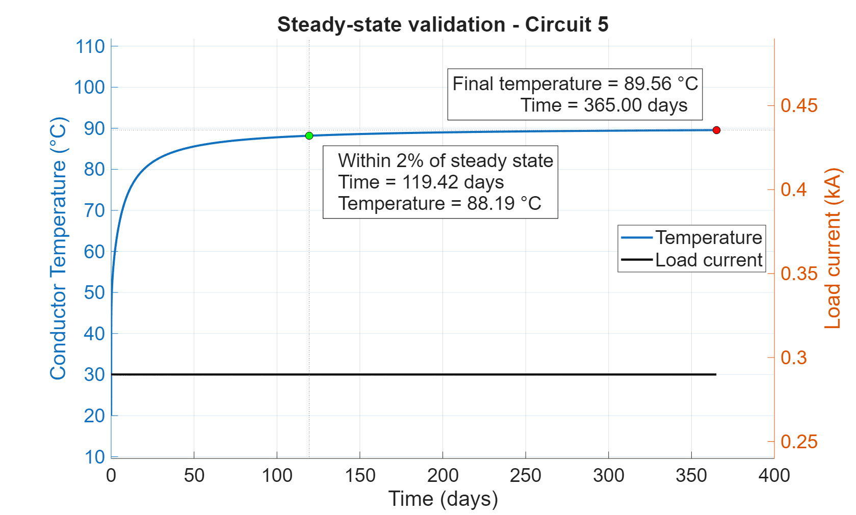
Figure 3 (a to e): Preloaded start, run to convergence (tolerance 0.1 °C). Daily peak settling, circuits 1 to 5.
Table 3: Settled peak conductor temperature and settling time (preloaded start, tolerance 0.1 °C).
| Circuit | Settled peak temperature (°C) | Setting time (days) |
|---|---|---|
| 1 | 50.11 | 38 |
| 2 | 51.71 | 38 |
| 3 | 52.17 | 38 |
| 4 | 51.70 | 38 |
| 5 | 50.10 | 38 |
No-load start (de-energised, conductor at 20 °C soil ambient). Each circuit starts from the native soil temperature, and then the cycle is applied. Day one peaks at ~38 °C, because the soil is cold and mutual heating between circuits has not developed. The daily peak rises as the soil warms and levels off by day 23:
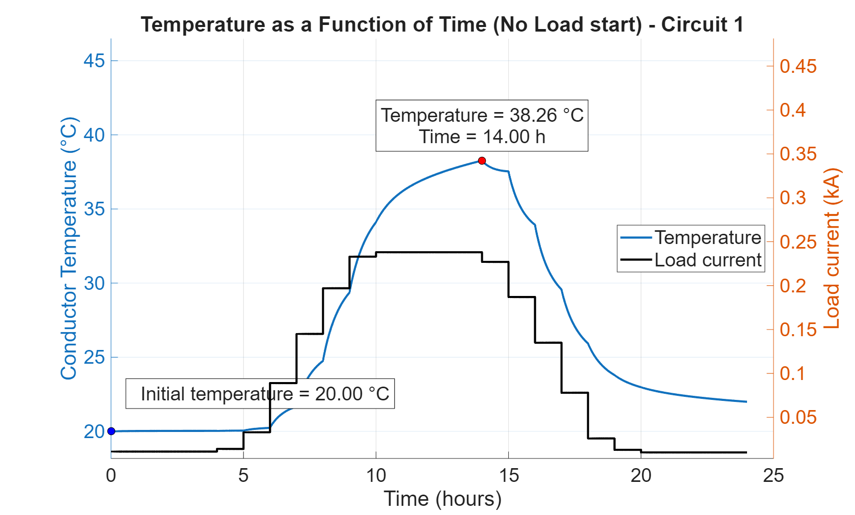


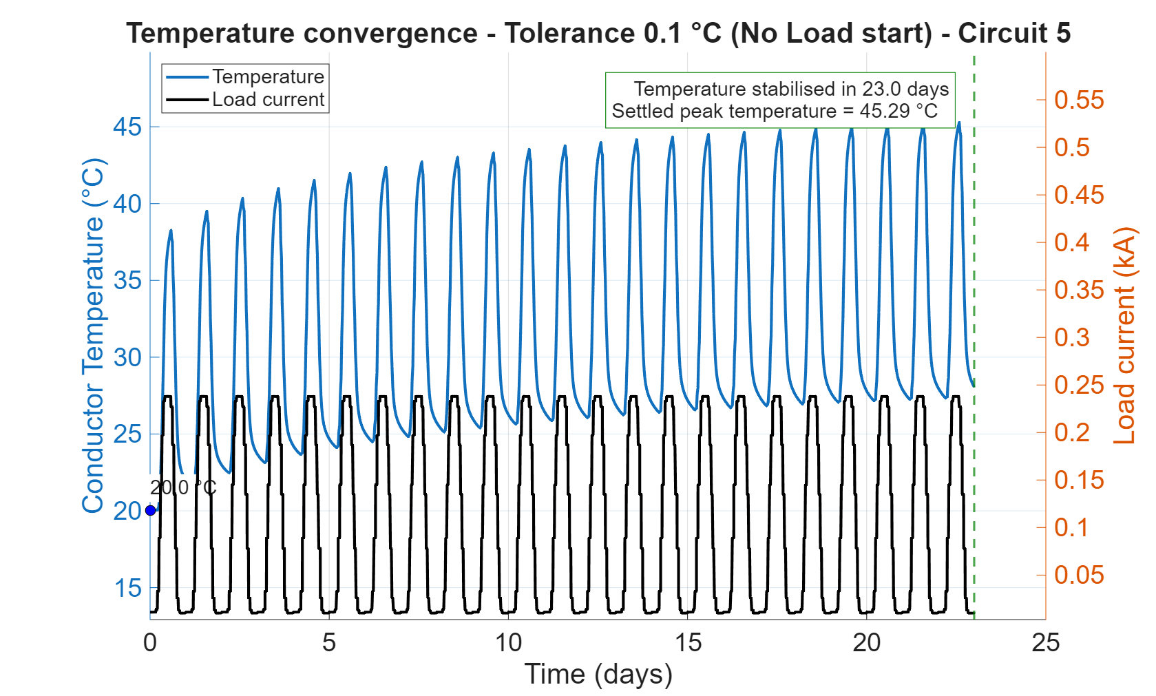
Table 4: Settled peak conductor temperature and settling time (no-load start, tolerance 0.1 °C).
| Circuit | Settled peak temperature (°C) | Setting time (days) |
|---|---|---|
| 1 | 45.30 | 23.0 |
| 2 | 46.75 | 23.0 |
| 3 | 47.20 | 23.0 |
| 4 | 46.74 | 23.0 |
| 5 | 45.29 | 23.0 |
Both cases are driven by the same load cycle, so they approach the same cyclic steady state: the preloaded start from above as the conductor cools, the no-load start from below as the soil warms. The converged peaks here (about 50 to 52 °C preloaded, 45 to 47 °C no-load) do not coincide because the stop criterion is a day-to-day change of 0.1 °C. The soil has a thermal time constant of weeks, so the daily change falls below 0.1 °C while the conductor is still approaching equilibrium, stopping each run early and bracketing the true value. A tighter tolerance closes the gap. Either way, a single 24-hour run under-predicts the long-term peak by nearly 10 °C in the no-load case because the soil continues to warm for weeks.
Soil dry-out
A single soil resistivity under-predicts conductor temperature. Soil next to a loaded cable loses moisture as it heats, and dry soil has higher thermal resistivity, often several times higher. A dry annulus forms next to the cable, surrounded by moist soil. A single-resistivity model omits this and overstates the available capacity.
IEC 60853-3 addresses this case (cyclic rating with partial soil drying), and the analytical dry-zone model of Mróz, Anders & Gulski (2023) applies the dry-soil resistivity beyond a critical interface temperature. Verify the soil model before relying on the additional capacity; if dry-out is credible for the site, model it or de-rate.
Emergency ratings
The same model gives the emergency rating: how much current a circuit can carry for a defined period, for example, two hours, after a parallel circuit trips, starting from a known pre-fault temperature. This is the emergency rating of IEC 60853-2.
Validation
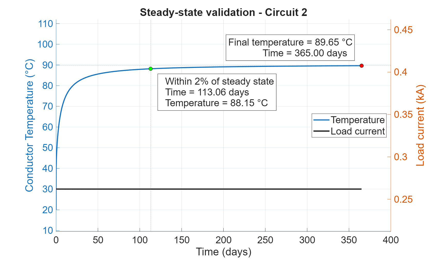
Holding each circuit at constant current to thermal steady state reproduces the IEC 60287 steady-state ratings above, confirming the transient model in the limiting case.


Practical takeaways
- The steady-state rating is not the usable capacity for cyclic duty; here, about 40 °C of conductor-temperature margin below the limit.
- Do not size from a single 24-hour run; iterate to the cyclic steady state. Settling takes 23 to 38 days here because of soil thermal inertia.
- Size the hottest circuit; interior cables retain more heat from neighbours on both sides.
- Verify the soil model; dry-out (IEC 60853-3) is the most common cause of an overstated dynamic rating.
- The same study gives emergency ratings (IEC 60853-2).
- Base the load profile on data covering the worst-credible period; a multi-step profile derived from historical data provides more capacity than a two-step or single-cyclic profile.
FAQ
Which load profile model gives the highest cable rating? Four are used: maximum continuous rating, single-cyclic profile, two-step profile, and multi-step profile. A multi-step profile built from several years of historical load or generation data provides the highest ampacity because it better represents the actual duty than a single bounding step. It is valid only if the data cover the worst credible period.
Why is a single 24-hour run not enough? The surrounding soil has a thermal time constant of weeks, far longer than the cable’s own. The daily peak rises over successive days until the soil reaches cyclic equilibrium, here at 23 to 38 days, so a one-day run under-predicts the long-term peak by nearly 10 °C in the no-load case.
What can make a dynamic rating inaccurate? Four inputs dominate: soil thermal resistivity and its seasonal variation, soil dry-out near the cable, mutual heating when circuits are closely spaced or touching, and a load profile that does not capture the worst-credible period. Any of these, if misstated, can remove the apparent margin.
Why does ignoring soil dry-out overstate capacity? Hot soil next to the cable loses moisture, and its thermal resistivity rises several-fold, forming a dry annulus surrounded by moist soil. A single-resistivity model omits this and overstates capacity. Account for it using IEC 60853-3 or the analytical dry-zone model of Mróz, Anders & Gulski (2023).
Does the starting condition change the answer? The preloaded (90 °C) and no-load (20 °C ambient) start bound the response and approach the same cyclic steady state, from above and below, respectively. Use them to bracket the result; with a loose convergence tolerance, they stop short and do not coincide.
Where is dynamic rating most valuable? On circuits with variable, peaky duty and high capital cost, especially offshore wind array and export cables, where conservative continuous sizing adds high cost. CIGRE TB 610 covers offshore generation cable connections.
Can the same method give emergency ratings? Yes: a short-time overload from a known pre-fault temperature (IEC 60853-2).
References
IEC Standards
[1] IEC 60287-1-1:2006+AMD1:2014 (Edition 2.0). Electric cables. Calculation of the current rating. Part 1-1: Current rating equations (100% load factor) and calculation of losses, General.
[2] IEC 60853-1:1985 (Edition 1.0, with Amendment 1:1994 and Amendment 2:2008). Calculation of the cyclic and emergency current rating of cables. Part 1: Cyclic rating factor for cables up to and including 18/30 (36) kV.
[3] IEC 60853-2:1989 (Edition 1.0, with Amendment 1:2008). Calculation of the cyclic and emergency current rating of cables. Part 2: Cyclic rating of cables greater than 18/30 (36) kV and emergency ratings for cables of all voltages.
[4] IEC 60853-3:2002 (Edition 1.0). Calculation of the cyclic and emergency current rating of cables. Part 3: Cyclic rating factor for cables of all voltages, with partial drying of the soil.
[5] IEC TR 62095:2003 (Edition 1.0). Electric cables. Calculations for current ratings. Finite element method.
CIGRE publications
[6] CIGRE Electra No. 87 (1983), WG 21.02. Computer method for the calculation of the response of single-core cables to a step function thermal transient.
[7] CIGRE Technical Brochure 610 (2015), WG B1.40. Offshore generation cable connections.
Paper
[8] M. Mróz, G. J. Anders and E. Gulski (2023). Soil dryout in the vicinity of cables with cyclic load installed in a backfill. IEEE Transactions on Power Delivery, 38(2).