0

Your Cart

0
Subtotal: AUD0
No products in the cart.
Home / Tutorials / Transient (Time-domain) Earthing & Grounding Grid Calculations

Transient (Time-domain) Earthing & Grounding Grid Calculations

ELEK SafeGrid Earthing V7.0
Downloads:

Table of Contents

Introduction

ELEK SafeGrid Earthing Software has a transient calculations mode which allows users to analyse theearthing response to a lightning waveform defined in the time-domain.

The transient calculations in SafeGrid can be used for:

  1. Determining the earthing response to lightning waveforms definedin the time-domain.
  2. Modelling standard transient waveform types including from IEC 62305, CIGRE, Heidler, Double-exponential waveforms as well as Custom waveforms from spreadsheets.
  3. Analysing the response in the time-domain which is displayed in plots versus time or animated with time 3D/2D surface plots (which can be downloaded as video files).

How to perform a transient calculation is explained with the following example as follows.

1. Sample earthing system

In this tutorial, the earthing system shown inFigure 1(drawn in AutoCAD) will be used for the transient calculations.The earthing system is a simple 10 m by 10 m grid with 1 m rods at each corner. The response to a lightning strike applied to the faulted segment will be calculated.
Figure 1– Example earthing system drawn in CAD

2. Design Settings

Start the transient calculation in Design Settings.

Figure 2 – Design Settings
  • Under Grid energisation. Select
  • Select either Current (A)or Voltage (V) as Grid energisation.
  • Specify Waveform and related parameters. SafeGrid supports severalstandard input waveforms and user-defined custom waveformswhich can be uploaded from spreadsheet files. 
Figure 3 – Input waveform types
  • IEC 62305 function: The function defined in the IEC standard is same as the Heidler function. The difference is that the steepness factor is a constant in the IEC standard. The correction factor, the peak current, the frontal and tail time constants are defined with respect to the following impulse shapes and lightning protection level.
    1. Impulse:
      1. First positive impulse (10/350 μs)
      2. First negative impulse (1/200 μs)
      3. Subsequent negative impulses (0.25/100 μs)
    2. Lightning protection level:
      1. LPL I
      2. LPL II
      3. LPL III – IV
  • CIGRE function: The CIGRE function has been introduced in section 3.9 of CIGRE technical brochure No. 063. The inputs to this method are the peak current (kA), the frontal time (μs), the decay time (μs) and the steepness of the wave (kA/μs). There is a lower limit to the value of the decay time which is calculated from the frontal time.
  • Heidler function: The inputs to this method are the peak current (kA), the frontal time (μs), the decay time (μs) and the steepness factor. The decay time must be greater than 1.135 times the frontal time.
  • Double-exponential function: The inputs to this method are the peak current (kA), the frontal time (μs) and the decay time (μs).
  • Custom from spreadsheet: The data in a tab delimited file can be imported into SafeGrid and used for calculations. The file formats can be any of the following:
    1. Only current values: The file will have only 1 column which contains the values of current. The additional input required in the user interface for this type of file will be the sampling time (μs).
    2. Time and current values: This file will have 2 columns, time and current. The time may or may not be uniformly sampled.

In this tutorial, we will use the following settings:

  • Waveform – IEC 62305 function
  • Impulse – First positive impulse (10/350 μs)
  • Lightning protection level – LPL II
Figure 4 - Example input waveform settings

3. Build Grid

Import the sample grid in Figure 5 to the Build Grid module.
Figure 5 – Build Grid
  • In Build Grid module press Import CAD and select the ASCII DXF file to import.
  • Setthe Drawing units with dropdown options or use the units that have been set in the drawing file
  • Import entities from All layers or the Layers selected. Hold Ctrl key to select multiple layers.
  • Import the grid in 3D by selecting Import 3D drawing units with Z-coordinates or in 2D by selecting Specify fixed depth.
  • Press Import to load the grid file.

4. Safety Criteria

Voltage profile(s) specify the area(s) where the actual surface and touch voltages will be calculated.

4.1. Add voltage profiles

  • Safety Criteria has a default rectangle profile. Click Fit to Grid to auto-size the voltage profile to cover the entire grid area.
  • To add a line profile, press Add Profile and specify Line as the profile type and press

Set the line profile to Fit to Grid to cover the entire grid area.

Figure 6 – Add Line Profile

4.2. Add grid points

Grid points specify the places on the grid where voltages and currents will be calculated.

  • To add grid points, switch to Grid points tab first on the side.
  • Click Add Point to add grid points at four corners of the grid.
  • Set the calculate mode to Voltage and Current for all of them
Figure 7 – Add Grid Points

5. Display Results

This module performs the transient calculation and displays results plots for analysis.
  • Click Calculate to obtain the result plots. The calculated Grid Impedance (Z) and Max. Grid Potential Rise (GPR) will also be displayed.
  • Click Pop-out to open the Input Waveform Preview which is helpful when comparing the output plots in the other tabs to the input waveform.
Figure 8– Display Results

The following are the transient calculation results:

Figure 9 – Input Waveform plot

Input waveform plot shows the lightning waveform defined in Design Settings. In this example, the IEC 62305 function is plotted.

Figure 10 – Faulted segment plot

Faulted segment plot includes the faulted segment voltage and impedance. The voltage (kV) versus time is plotted which has the same shape as input waveforms. The impedance magnitude (Ω) and phase angle (°) are plotted against the frequency (Hz).

Figure 11 – Maximum surface voltage (kV) during the response of the rectangle profile
Figure 12 – Maximum surface voltage during the response along the line profile

The animated plots show the surface voltages on the grid and along the line profile during the response.  With reference to the pop-out input waveform, you canjump to the moment in time of maximum surface voltage. The response can be downloaded as a video file.

Figure 13– Maximum touch voltage (kV) during the response of the rectangle profile
Figure 14– Maximum touch voltage during the response along the line profile

The animated plots show the touch voltages on the grid and along the line profile during the response.

Figure 15 – Grid point response at faulted segment

The grid point plot shows the voltage and current at Grid Point 1 (0 m, 0 m) close to the faulted segment. Negative current signifies a negative direction in current flow from the end to the start of the segment.

Figure 16 – Grid point response away from faulted segment

The grid point plot above shows the voltage and current at Grid Point 2 (10 m, 0 m) away to the faulted segment.

The voltage and current at Grid Point 3 and 4 are similar as Grid Point 2.

Related Tutorials:

This tutorial shows how to use the Fault Current Distribution module in ELEK SafeGrid Earthing Software to model an earth fault on an overhead transmission line with an underground cable link.
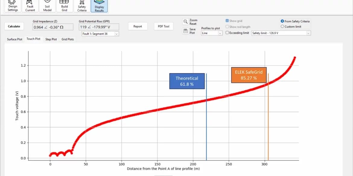
With the Fall of Potential Test, the resistance of an earthing system is measured using a remote earth electrode. There is a theoretical position of 61.8 % of the separation distance between the measured grid and the remote electrode, which is the correct position for measuring the exact grid impedance for uniform soil resistivity but not for multilayer soils. This tutorial shows ELEK SafeGrid Earthing Software users how to simulate an FOP test.
This video tutorial focuses on the design and modelling of Earthing Systems for Wind Farms and Solar PV Farms. Real-world examples are provided and are explained.
SafeGrid can model custom earthing arrangements of any size or shape in 2D or 3D. You can specify the grid using the in-built editor tools or you can import grids drawn in AutoCAD.
This video (25 min) tutorial shows the main features of SafeGrid Earthing Software for performing an earthing designs and explains the design process.
Example Rolling Sphere Method calculation which shows how to overlay protection systems such as lightning masts and earth wires on a site drawing.