Table of Contents
Introduction
IEC 60287 often overestimates cable ampacity for shallow-buried HV cables because it ignores soil–air cooling at the ground surface. A new method that corrects this by modelling real soil temperature effects is explained and compared with traditional IEC calculations and the finite element method.
Cable Ampacity Calculation Error: IEC 60287 Isothermal vs Non-Isothermal Ground Surface
The IEC 60287 standard is the internationally recognised method for calculating underground power cables’ current-carrying capacity (ampacity), constituting approximately 67% of all cable systems worldwide [ref. 1]. The maximum permissible conductor temperature limits cable ampacity, as excessive heat accelerates insulation degradation and significantly reduces operational lifespan. IEC 60287 employs the Kennelly hypothesis and method of images to calculate external thermal resistance, assuming the soil-air interface remains isothermal at ambient temperature. While this isothermal assumption simplifies thermal analysis, it neglects the convective heat transfer mechanisms at the ground surface. For deeply buried cables, this simplification provides reasonable accuracy; however, a recent study by National Grid in the United Kingdom demonstrates that it can substantially overestimate ampacity for shallow installations, potentially compromising cable reliability and safety margins [ref. 2].
This article presents an analytical method that accounts for the non-isothermal ground surface by incorporating convective heat transfer at the soil-air interface. We compare the ampacity results from this analytical approach with those obtained using the finite element method—which provides the most accurate representation of non-isothermal surface conditions—and with the standard IEC 60287 method, which assumes an isothermal ground surface. This comparison demonstrates how the isothermal assumption can lead to overestimation of cable ampacity and validates our analytical method as a more conservative and reliable alternative to the current standard.
ELEK Cable HV Software has been used for the modelling and calculations.
Case Studies
Case Study 1
The study compares ampacity using the IEC isothermal (idealistic), IEC non-isothermal (analytical), and Finite Element (FEM) methods. It uses a single-core 132 kV, 1200 mm² Copper round stranded conductor with a wire screen and a foil sheath. The cable is solidly bonded and directly buried. The installation conditions are given below.
| Parameter | Value | Unit |
|---|---|---|
| Soil temperature | 20 | °C |
| Soil thermal resistivity | 1 | K.m/W |
| Air temperature | 40 | °C |
| Arrangement | Trefoil, touching |
The calculation results from the IEC (isothermal) method, IEC (non-isothermal) and FEM method are compared. The cable’s depth is varied, and the current ratings are noted.

Case Study 2
The study investigates the effect of the air temperature above the soil surface on the cable’s ampacity. The cable model above is used, and all conditions as in case study 1 are maintained. The air temperature varies from 25 °C to 40 °C, and the circuit is buried at 0.7 m.

Key Takeaways
The following points are observed in the case study:
The calculations with the IEC 60287 overestimate the ampacity at shallow depths due to the assumption of isothermal conditions.
As the air temperature above the soil increases, less heat is transferred from the cables to the air, which increases the cable’s temperature.
For cables shallowly buried, the ampacity overestimation leads to higher cable temperatures.
The difference between the IEC isothermal and non-isothermal current ratings for deeply buried cables is reduced compared to shallow-buried cables.
The results of the IEC non-isothermal modelling are in good agreement with the FEM results.
Theory
IEC 60287 Method: The Isothermal Earth Surface Assumption
The lifespan of underground cable insulation is directly determined by the maximum temperature reached by the conductor. This temperature is a function of the current, the cable’s construction, and the thermal properties of its environment.
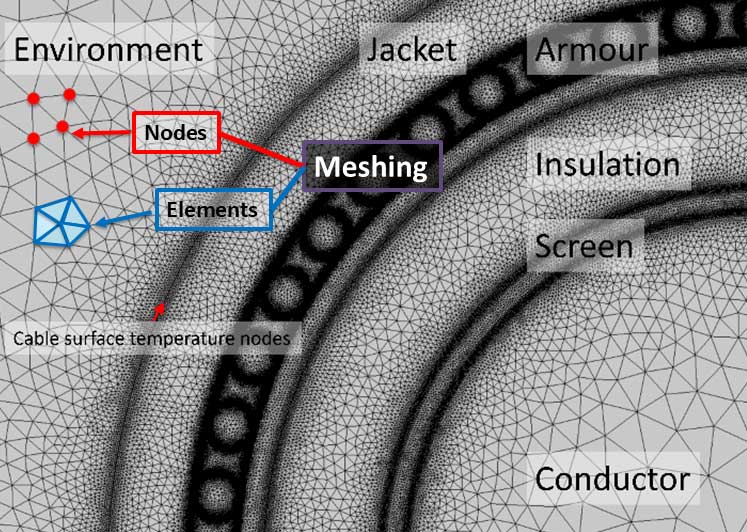
A critical component of the thermal circuit is the external thermal resistance (T4) in K.m/W, which models the heat flow from the cable to the ambient air. The standard calculates T4 using images, also known as the Kennelly hypothesis. In this method, the real heat source (the cable) is mirrored in an imaginary plane above the soil to account for the soil–air boundary. The sum of temperature rises caused by the real cable and its fictitious image gives the temperature at any point in the soil.

The IEC method uses the following:
Isothermal boundary – the soil‑air interface is assumed to have a uniform temperature equal to the ambient air temperature. Convective cooling is neglected; only conduction through the soil is considered.
External thermal resistance—IEC formulas calculate T4 based on soil thermal resistivity, burial depth, and cable geometry. The standard method uses fixed coefficients and logarithmic expressions derived from the image method.
Kennelly’s hypothesis: Thomson (Lord Kelvin) and Kennelly’s image method is used for electrostatic and thermal problems.
This mathematical technique simplifies the problem by replacing the soil-air interface with an imaginary, perfectly conducting plane (an isotherm). For every real heat source (the cable) buried at depth L, an imaginary heat sink is placed symmetrically above the ground at a height L. The rise in temperature at any point in the soil can then be calculated as the sum of the effects of the real source and its image.
The Limitation: While mathematically convenient, this method inherently assumes the Earth’s surface has a fixed, uniform temperature. Because convective cooling is ignored, this method overestimates the cable’s ampacity for shallow burial. Finite‑element studies have shown that assuming an isothermal surface can produce conductor‑temperature predictions significantly lower than reality for cables buried up to 1 m [ref. 3].
 lies within the soil.")
Importance of considering the non‑isothermal surface
Avoiding over‑estimated ampacity
Experimental and numerical studies demonstrate that ignoring convective cooling leads to optimistic ampacity ratings. For cables buried at 0.5 m, the temperature difference between conventional fixed‑temperature and convective boundaries is around 6.5 %. IEC formulas using the isothermal assumption yield ampacity values that are too high for shallow installations. Such overestimation risks overheating cables, reducing insulation life and increasing failure probability.
Enhanced accuracy for design and operation
Modelling the soil–air interface as a non‑isothermal boundary makes the calculated conductor temperature closer to reality and ensures safe cable design. The approach is critical when:
Shallow or variable burial depth – installation depths less than 1 m result in significant convective cooling. A non‑isothermal model prevents underestimating the external thermal resistance.
Transient loading or high losses – natural convection becomes more pronounced as surface temperature rises. Accurate convection coefficient calculation ensures that seasonal and loading variations are captured.
 crosses the soil boundary.")
Differences between isothermal and non‑isothermal soil surfaces
| Aspect | Isothermal surface | Non‑isothermal surface |
|---|---|---|
| Boundary condition | The soil-air interface is kept at the soil temperature (ambient temperature, no convective heat exchange). | The convective boundary layer at the soil surface exchanges heat between the ground and the ambient air. |
| Modelling approach | Method of images with a fixed plane; thermal resistance T₄ computed directly from geometry and soil resistivity. | Introduces a fictitious layer of thickness to account for the non‑isothermal boundary; the cable is treated as if it is buried deeper, and the convective heat‑transfer coefficient is calculated iteratively. |
| Heat‑transfer processes | Only conduction through soil is considered. | Both conduction through soil and natural convection at the soil‑air interface are considered. |
| Accuracy for shallow installations | Overestimates ampacity because convective cooling is ignored; error ≈ 6.5 % at 0.5 m burial. | Provides more accurate conductor temperatures; differences decrease as burial depth increases (≈ 4 % at 1 m). |
| External thermal resistance | Highest | Lower due to convective cooling; T4isothermal>T4fictitious layer>T4non‑isothermal. |
Methodology: The Fictitious Layer Model
The fictitious layer model integrates seamlessly with the established IEC 60287 framework. It models the convective cooling effect by adding a fictitious layer of soil of thickness d (m) on top of the actual soil surface.
The derivation uses the Fourier transform to convert the two‑dimensional heat‑transfer problem into a one‑dimensional diffusion equation. This fictitious layer has the same thermal resistivity as the soil. Its purpose is to effectively increase the burial depth of the cable in the image method calculation, thereby increasing the external thermal resistance (T4) and resulting in a more conservative (higher) conductor temperature calculation for a given current.
The core of the problem is calculating the correct thickness of this layer, which is a function of the soil’s thermal resistivity and the heat transfer coefficient of air.
Fictitious Layer Thickness
The Fourier‑domain solutions for the isothermal and non‑isothermal problems yield the relationship between the fictitious layer thickness d, soil resistivity ρ and heat‑transfer coefficient h (W/K·m²).

After the iterations have converged, the fictitious layer thickness is calculated as
\(d = \frac{1}{\rho h} \ \ \ \ \ m \)
Heat transfer coefficient of air
The heat transfer coefficient is computed using the maximum temperature of the soil surface via an integral equation method. The position of the fictitious image is obtained using the Fourier transformation. The final expressions are simple, and the layer thickness is compatible with the IEC standard method.
The Fourier transform converts a directly buried cable’s 2D heat transfer problem into a 1D problem.
\(\mathbb{F}\{T(x,y)\} = \bar{T}(s,y)\)
x and y are the horizontal and vertical coordinates,
s is the horizontal component in the Fourier domain.
Consider a cable with Qs (W/m) losses directly buried in the soil of thermal resistivity ρ. The cable is placed at a burial depth L (m) from the surface exposed to an ambient air temperature Tair. A cable can be considered a point source when compared with the vast expanse of the soil region.

Hence, the heat source could be expressed as a Dirac-delta function δ(x) at depth L from the surface, where the heat flux is Qs only at the cable’s position and zero elsewhere. The Dirac-delta function’s Fourier transform is 1.
\(\mathbb{F}\{\delta (x)\} = 1\)
This indicates that a straight line with constant heat flux in the Fourier domain can represent a cable in the space domain. The temperature at the surface, Tsurface, is a function of x, with the maximum temperature directly above the cable (x = 0) and gradually decreasing as one moves away \(\begin{aligned}
\overline{T_{surface}}
\end{aligned}\). can be computed iteratively to satisfy the heat equation at the soil surface
\(\overline{T_{surface}} = T_{amb}+\frac{Q_s}{\overline{h}}\)
\(\overline{h} = \frac{Nuk}{L_c} \ \ \ W/m^2K\)
Nu is the Nusselt number
k is the thermal conductivity of air
The value of h obtained from the above equations is independent of cable depth and dimensions. It depends only on the physical properties of air and the amount of heat dissipated. An iterative procedure is used to reach a final value of h.
Conclusion
The IEC 60287 standard traditionally assumes an isothermal soil surface, leading to simple analytical formulas for the external thermal resistance. This assumption ignores convective heat exchange at the soil‑air interface and can overestimate the ampacity of buried cables. Modelling the soil surface as a non‑isothermal boundary introduces a convective heat‑transfer coefficient and a fictitious soil layer whose thickness depends on soil resistivity and air convection. The fictitious soil layer is modelled using the Fourier transform and is compatible with IEC 60287. This modelling significantly improves the accuracy of ampacity calculations for non‑isothermal soil surfaces. Therefore, the non‑isothermal surface is essential for reliable cable‑rating assessments and ensuring underground power cables operate within safe thermal limits.
References
IEC 60287-2-1: “Electric cables – Calculation of the current rating – Part 2-1: Thermal resistance – Calculation of the thermal resistance”.
National Grid Electricity Transmission, “Rating Impact of Non-isothermal Ground Surface (RINGS),” Network Innovation Allowance Project NIA_NGET0082, Energy Networks Association Innovation Portal, Apr. 2012–Jun. 2016. [Online]. Available: https://smarter.energynetworks.org/projects/nia_nget0082
CIGRÉ Working Group B1.49, “Installation of Underground HV Cable Systems,” CIGRÉ Technical Brochure 889, CIGRÉ, Paris, France, 2022.