The Earthing Design Process using SafeGrid
SafeGrid Earthing Software is finite element-based calculation software that is easy to use and accurate for designing safe earthing and grounding systems.
In the SafeGrid user interface the buttons at the top are the main modules of the software. You can switch between the modules at any time.
Generally, the design process would be from left to right starting at Design Settings and working through each of the modules as required, entering data, until you reach Display Results where you would calculate the performance and safety of the earthing system. If after calculating the results you need to change the design, then you can return to any of the modules, make the necessary changes and re-calculate the results.
In this tutorial we will go through each module of SafeGrid including the reports, and show you the software features and explain how they work. If you have any questions along the way, we recommend you note them down, then you can discuss those with our engineering team over email or a call which you can schedule.
Design Settings module

For a new project, you would start with the Design Settings module which allows you to set much of the preliminary inputs of earthing system design, such as the Soil characteristics, Grid energisation, Conductor types, and Decrement factor.
Firstly, we should look at the Soil characteristics. The soil characteristics allow you define the soil model. SafeGrid can model multi-layer soils which is important because most soil structures are multi-layered. The soil model used for your designs is incredibly important and will have a significant impact on the results. You can enter the soil model explicitly, or you can use the results from the soil model module, which I will show you in another section of the video.
You can modify the number of layers, the resistivity and thickness of each layer, relative permittivity, and the frequency dependency method, which enables you to select a particular frequency dependent soil model. Note that the last soil layer does not have a defined thickness, as it is assumed to have infinite thickness.
Next, the Grid energisation section is where you can define the earth fault current. You can enter the values explicitly, or you can use the Fault Current distribution module which we will explore soon. Earth fault current level can be entered as either a current or a voltage with a real and imaginary magnitude. Additionally, the frequency of the energisation can be defined, and this will determine which frequency dependency methods are available to use under soil characteristics. Note that soil electrical resistivity and permittivity (both used for the calculations) vary significantly with increasing frequency. SafeGrid can model up to high frequencies up to frequencies suitable for modelling lightning currents. There are technical articles at our website to guide you on how to model lightning currents.
You can also add various Conductor types. SafeGrid uses an advanced algorithm that considers series voltage drop and impedances of all conductors in the network. You can add or remove conductors and change the description and size of each conductor. By default, there are two conductor types included in the project, one for the main grid conductors and another for the rods. If you press ‘calculate minimum size’, a prompt will come up that will allow you to change the material of the conductor and determine the minimum size and the rating, per the IEEE Standard method.
Finally, you can calculate the Decrement factor, which is the DC offset of the fault current and will affect touch and step voltages of the earthing system.
Fault Current module

Moving on to the Fault Current module. You can use this module to determine an accurate earth fault current also known as ‘split factors’ for your earthing system. Typically, the actual fault current which enters a grid during a fault is significantly lower than the maximum prospective fault level.
Fault current distribution can be difficult to analyse, but SafeGrid Earthing software makes it easy for you to calculate. There are sixteen (16) standard cases provided ranging from cables to overhead transmission line connections. For cable supplies there are cases for single core and multicore cables with different bonding arrangements including solid, single point or cross-bonded screen arrangements. There are also overhead transmission line cases with single or double overhead earth wires and multiple tower sections can be modelled.
Once you have selected a standard case a schematic diagram is displayed where the circled numbers are the nodes, and the lines are the conductors of the electrical network. A short-circuit is simulated between a single-phase conductor and the local earth grid, or the grid under study which is shown as “EG LOCAL”. At the node where the fault is applied the fault current splits between the local earth grid and the conductive return paths such as the cable screens. In the case shown here only 4% of the total fault current enters the local earth grid giving rise to touch voltage hazards.
Once you have selected from the standard cases you can enter basic data inputs to match the feeding supply, such as fault current level, cable length, soil resistivity, earth grid resistance, phase conductor positions (for mutual impedance calculations), and the electrical properties of the conductors.
It’s also possible to model multiple supplies connected to the local earth grid and feeding the fault by adding and configuring multiple standard cases. Once this is done, you can press the calculate button to calculate all the current distributions in the system and determine the local earth fault current level.
Calculating fault current distribution can often result in much lower touch voltages making it easier for you to achieve safety compliance – saving you time and money both during the design and the construction.
Soil Model module

Moving onto the next module, which is Soil Modelling. As mentioned back in the design settings, you can enter the soil model explicitly, or use the soil model module. In this module, you can add multiple data points of Wenner soil resistivity measurements. You can add as many measurements as you’d like and change the spacing and the value that was measured of each data point, which can be in resistance or resistivity. You can then calculate the multilayer soil model. It’s also possible to analyse multiple datasets or traverses. We recommend that you use multiple datasets, as this will allow the most accurate soil model possible to be generated.
You can also import measurements from a spreadsheet file, such as a CSV file. I will import a dataset of soil resistivity measurements, which contains 13 measurements, with spacings ranging from 0.5 metres up to 54 metres. I will set the number of soil layers to 3 and calculate the results of the soil model. You can set the model to have any number of layers that you wish, but SafeGrid will only give you up to a certain maximum number of layers that it can detect.
I’ll now set the number of soil layers to two and re-calculate. This is a good example of why you need multi-layer soil capability. Looking at this plot, the crosses represent each of the measured data points from the Wenner measurements. The black curve represents the apparent resistivity curve which is the fitted model. Judging by the distribution of the black crosses, we can see that a two-layer model is not a great fit, because the resistivity starts low, rises to a peak, and then goes back down, which suggests there are at least 3 layers.
In the results section, we can see the RMS error, or goodness of fit, of the model is 28.26% which is quite a high error. If we set the number of layers back to 3, we can see that the RMS error decreases to 6.77 %, which is significantly lower. Additionally, we can see the fitted line of the model lines up well with the data. A low RMS error means we can have a high confidence that the field measurements and the model are well-matching.
We can sometimes improve the goodness of fit between the measurements and the model by excluding outliers. While it may not be extreme in this case, we can see certain points on the plot that could be considered outliers for this plot, as in they sit far away from the calculated apparent resistivity curve. Counting backwards from the largest spacing, we can see the most apparent outlier is the 10th data point, or R10. If we exclude this measurement and re-calculate, we get a better RMS error (better being lower), of only 4.49% compared to the previous 6.77%
You can also account for driven probe depth for short spacings, generally at 2.5 metres spacing or less. Enter the driven depth of the probe during the Wenner measurements, and SafeGrid will automatically adjust the model based on the depth that you’ve entered.
Building the Grid

Next, we have the Build Grid module which is used to design the layout of the grid.
The grid display shown here is from a top-down X and Y view, or a 2D plan view, there are also other views. By default, the grid shown is 30 metres by 30 metres grid which is buried at 0.5 metres. You can adjust the view of the grid. ‘Equal scaling’ makes the X and Y scale the same, whereas ‘Fit area’ makes the grid span across the whole plot. Which view you use is based on your preference.
SafeGrid can model grids of any size or shape, including very large or complicated grids, and you can add multiple grids into the same model which are not interconnected. You can build the grid model using the in-built grid drawing tools, of which there are many, additionally you can import earthing grids drawn using 2D or 3D AutoCAD.
I’m going to show you how to import an AutoCAD file. When you import a CAD file, a window pops up. You can see the path to the file. You can also see the drawing units of the file. You need to know the units for the purposes of calculation. Normally the drawing units are set in the AutoCAD project file and SafeGrid can read them, but if they aren’t set, you can set them manually here in this window.
All the drawing layers in the CAD file are shown in the table. You can select to import layers from all layers or only from selected drawing layers such as those relevant to the earthing system.
For a 3D CAD drawing, you should select “Import 3D drawing with Z-coordinates” so that the depth is also plotted. This file shown here is a grid model for a wind turbine foundation which was drawn in CAD and imported into SafeGrid for modelling.
SafeGrid will check the grid for overlapping conductor errors and help you to resolve them since they may possibly cause errors.
There are other views such as the orthographic view which gives a 3D perspective of the grid model. We can see that the wind turbine model has parts that are above ground, or Z = 0, and below ground. SafeGrid can model grid conductors which are buried or above the ground surface.
I’m going to import a CAD file for a solar farm earthing system to show what the software is capable of modelling. This is another file drawn in 3D CAD, as each of the supports for the solar panels have been modelled. Generally solar farms are quite complicated with lots of conductors, but SafeGrid is a powerful enough software to be able to deal with many thousands of grid conductors.
I’ll also import a substation earthing system. I’ll select these two layers that are directly related to the earth grid, and I’ll also show what it means to have a background layer. This is the layout of a 110 kV substation. The greyed-out conductors are “background” conductors, which means that they signify the location of a building which we will see when we calculate the results.
The faulted segment can be moved to any location on the grid. The faulted segment is where the fault current will be applied during the simulations. For meshed grids or for small grid dimensions, the fault location makes little difference to the results but for large or radial networks the fault location can affect results significantly.
You can make modifications to the grid using the in-built drawing tools which function similarly to the tools in AutoCAD. There are snap tools for drawing which can be switched on or off.
I’m going to show you how to add rods to the substation earth grid. From the Drawing Tools drop-down menu select “Add Rod”. A message is displayed in the bottom left corner with instructions to specify the rod length which I will enter as 5 metres. Next, you can move the mouse of the grid and left click the mouse to add rods at any point. Once you’re finished adding rods you can press Escape.
Let’s look at the Conductor Type View. This shows all the various conductor types in the grid. We can see the conductors of the main grid, and all the rods that we just added. Next, let’s look at the orthographic view once again. We can see the added rods at these points as well.
There are tags that can be used to assign conductors to various groups. You can switch different groups on and off for calculations, so that you can test various scenarios. Conductors can also be set to be insulated. Right click the desired segment, highlight “conductor type”, and click “insulated”.
Any modifications we make to the earthing grid can be exported back into AutoCAD.
Safety Criteria

Let’s move on to the Safety Criteria module which has two main sections: the “voltage profiles” tab and “safety criteria” tab.
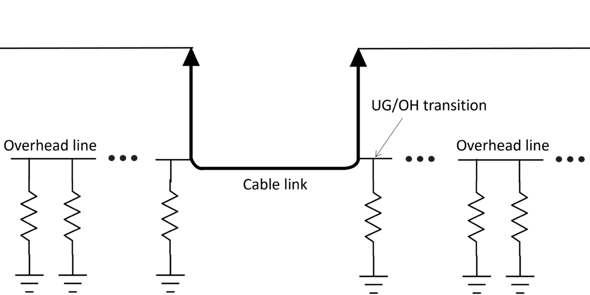
The Voltage Profiles tab includes the controls for you to specify the locations where you will calculate the surface, touch, and step voltages with respect to the earthing grid location. A voltage profile is displayed as a rectangle which can be manually re-sized or can automatically be fitted to the entire grid by pressing ‘Fit to grid’. There are points, or dots, that can be seen throughout the rectangular profile. Each one of these points is where surface, touch and step voltages will be calculated. You can have multiple voltage profiles and overlap them in case your grid is an odd shape. You can also add a line profile, and the touch and step voltages will be calculated along the line rather than over a rectangular area.
You can adjust the maximum spacing between each point. By default, this value is 2 metres. You should adjust the spacing between points to be reasonably small but not too small such that it generates an unnecessary number of points. The spacing between points affects the appearance of the final plots but also affects calculation times. The SafeGrid algorithms are fully optimised so generally it does not take a long time to perform calculations, however if the spacing between points is too small, the calculation time could be excessive. We recommend starting with a larger spacing, and once you are happy with the designs, you can recalculate results with smaller spacing for nicer plots with higher resolution.
There is a Touch Voltage Reference area. By default, touch voltages are calculated with respect to the grid potential rise, but you can also calculate touch voltages with respect to reach distance, among other reference modes.
The Safety Criteria tab is where you can specify the touch and step voltage, or safety, limits. By default, there is an allowable touch voltage and an allowable step voltage, denoted by two curves in this plot.
The plot shows allowable maximum voltage versus time. The blue curve is for touch voltages, and the red for step voltages. As you can see, touch voltage limits are normally lower than step voltage limits.
You can adjust the fault clearing time. When you reduce fault clearing time, which means you’re clearing the fault faster, then allowable touch and step voltages go up.
SafeGrid can perform safety limit calculations in accordance with the IEC standard or the IEEE 80 standard. If you change the standard, you can see that the curves will have a different characteristic shape this is because the theory and principles behind these two standards are very different. The IEEE standard is based on the 50 kg and 70 kg body weights and a standard fixed body impedance value of 1000 ohms.
The IEC standard method is more advanced than the IEEE standard. Instead of just touch or step voltages for the body current path, you can have a custom body current path, and custom heart current factors, body current factors, etc. These are advanced settings used for customisation. For the IEC method, we can set the fibrillation current probability, body resistance, dry or wet conditions, and the conversion factors, which are explained in the manual.
You can also include an additional surface layer such as a layer of crushed blue metal rock that can be applied to the safety limits. Foot resistance is automatically calculated, but you can also add additional shoe or glove resistance.
The safe limits that you specify in the Safety Criteria module become available in the Display Results module so you can compare them with the actual grid performance to assess safety.
Display Results module - Analysing Surface, Touch and Step Voltages

The final step in the process is to go to Display Results and to calculate the results.
When you press Calculate, a summary of inputs will appear. This allows you to do a quick check of the most important parameters of what you’re going to calculate, such as number of layers, soil model parameters (here I am using the results of the soil model module), the earth fault current level, decrement factor, number of conductors, etc. You can optionally calculate step potentials, although this will take a little more time.
Once you press calculate, the program will take a short amount of time to perform the calculations of the grid. The software will firstly calculate grid impedance and grid potential rise. We can also see that there have been several detailed plots which have been generated.
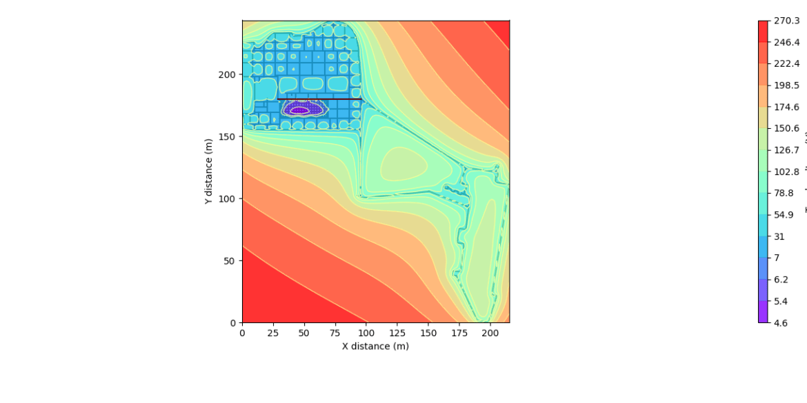
The first plot is the Surface Plot, which is an interactive plot. What’s shown here are the ground surface voltages of the grid, ranging from the maximum voltage to the minimum voltage. You can also see the grid displayed underneath the plot. The legend down below denotes the various segments of the grid, such as the faulted segment, rods, and background segments.
If desired, you can look at the plot in 2D. Whilst 3D plots are attractive, 2D plots are generally more useful for designing. You can zoom and pan the plot. When you move your mouse cursor over certain points, you get the exact voltage at that point.
Other generated plots include the touch voltage plot and the step voltage plot in both 2D and 3D. Additionally, three grid plots are generated.
The first grid plot shows the leakage currents of the system. SafeGrid calculates the exact values of all the currents which are leaking out of the conductors and into the soil. You can click on each conductor and see the current value and phase angle. The range of currents is displayed here. All the leakage currents should add up to the total fault current of the system.
The second grid plot shows the longitudinal currents. These are the currents that travel along each conductor. The faulted conductor will have the highest magnitude of longitudinal currents. As the fault current is dispersed throughout the meshed grid, the longitudinal currents should reduce.
The third grid plot shows the segment voltages. As mentioned earlier, SafeGrid uses a very advanced algorithm which considers the series voltage drops along all the conductors in the grid. The segment voltages plot shows the series voltage drops along each conductor in the grid. The highest voltages are at the fault location, and they are slightly lower the further the conductor is from the fault. In this grid, the voltage difference from the maximum to the minimum is small, only about 2.2 V, but that can be a much bigger difference for a radial style grid, or grids in low resistivity soil. Series voltage drops are very important to consider.
Going back to touch voltages, one of the main objectives of the software is to determine whether the touch voltages exceed the safety limit determined earlier. If we tick “Exceeding limit”, we can see all the areas which have touch voltages that exceed the safe limit. In most cases, we are only interested we are only interested in areas that are within the grid or within 1 metre away from the grid. It’s possible to update the safety criteria or modify the grid and recalculate the results to better fulfil the safety criteria.
SafeGrid includes a comprehensive report generation tool, in either PDF or Word format. You can show your own company logo on the report, and the report is fully customisable. You don’t necessarily need all the data. If you need the raw table data, it can be exported from the “Tools” menu.
Let’s look at the report for this calculation. As you can see, the report includes all the input data, such as the design inputs, like the soil model. The fault currents, conductor types, frequency, soil measurement inputs and calculated soil model are all included as well.
Conductor size calculations and grid model (including imported layers if applicable) are also shown. A bill of materials, which breaks down all the characteristics of the conductor types, along with a plot showing each of the different conductors is included in the report.
The safety criteria calculation inputs and limits for touch and step voltages can also be found in the report. The voltage profiles and touch voltage references can be seen in the report too.
Finally, the calculated results from the Display Results section can be seen, such as the Grid Impedance, GPR, and the various calculated plots in both 2D and 3D. You can also see the plot from the line profile that I created earlier on in the video.