Downloads:
Benefits of determining fault current distribution
The touch and step voltages associated with an earthing system are directly proportional to the magnitude of the fault current flowing into and directly discharges into the soil by the earthing system. Therefore, it is important to determine how much of the fault current returns to remote sources via the cable screens or the overhead earth wires of the lines feeding the substation.
In many cases, the portion of the fault current discharged into the substation earthing system will be lower (often substantially lower) than the maximum fault current available. This is the significant benefit of determining the actual fault current distribution.
If you can show that the fault current entering your earthing grid is significantly lower than the maximum fault current (often the case) this will dramatically reduce touch and step voltages (the requirements) and greatly simplify the design.
To determine the actual fault currents, it is necessary to calculate the overhead line or cable line parameters such as the self and the mutual inductive and capacitive impedances but also to know other parameters at the representative locations.
Using the FCD module
The Fault Current Distribution (FCD) module in SafeGrid is for calculating the actual fault currents. The FCD module uses an accurate Node Voltage (NV) calculation method flexible enough for calculating custom electrical network and earthing configurations.
There are 16 in-built standard cases of the FCD module representing various connection situations between two substations. There are 4 main groups to these 16 standard cases:
- Solid/single-point bonded Single-Core (SC) cables
- Individual/overall screened Multi-Core (MC) cables
- Cross-bonded single-core cables with/without earthing conductors
- Overhead lines
A description of each standard case is given by the drop-down menu and a schematic diagram of the arrangement which is being modelled is previewed.
The steps to use FCD module is simple.
- Select from the standard cases for modelling standard arrangements for substations
connected by either cables or overhead lines. - Input the necessary data regarding the case you have selected.
- Calculate the fault current distribution results and use them for later calculations of touch and step voltages.
Single phase to earth faults are assumed for the standard cases.
Note if there are multiple connections (sources of fault current) to the local earth grid (that which is under study) exist then multiple individual calculations may be undertaken using the FCD module and superposition is used to determine the total fault current.
Example systems
In this tutorial two example systems will be investigated to show how to use the FCD module.
- System A – Two substations connected via underground cables
- System B – Two substations connected via overhead transmission lines
In the following examples calculations we will consider two substations A and B connected by either cable or overhead line if there is fault at Substation A what portion of the fault current will flow into the earth grid giving rise to possible touch and step voltage hazards. In the models only the faulted phase and the earth return conductors such as overhead earth wires and cable screens need be considered.
A single phase to earth fault level of 7 kA and a soil resistivity of 100 Ω.m was used for both systems.
System A - Two substations connected by screened underground cables
The first example system consists of 22 kV 630 mm2 single-core cables with solid-bonded screens connected between two substations which are located 913 m apart.
The cables installation arrangement is shown in Figure 1. The cables are installed in a backfilled trench buried at a depth of 0.7 m in a 0.2 m flat-spaced formation.

The cables bonding arrangement schematic diagram is shown in Figure 2.
The physical and electrical characteristics of the cables are shown in Table 1.
Table 1 – Characteristics of the 22 kV, 630 mm2 solid-bonded single-core cable
| Conductor diameter | Diameter over wire screen | Screen thickness | Conductor AC resistance | Screen AC resistance |
|---|---|---|---|---|
| 29.9 mm | 47.2 mm | 4.5 mm | 0.0388 Ω/km | 0.2893 Ω/km |

System B - Two substations connected by overhead transmission lines
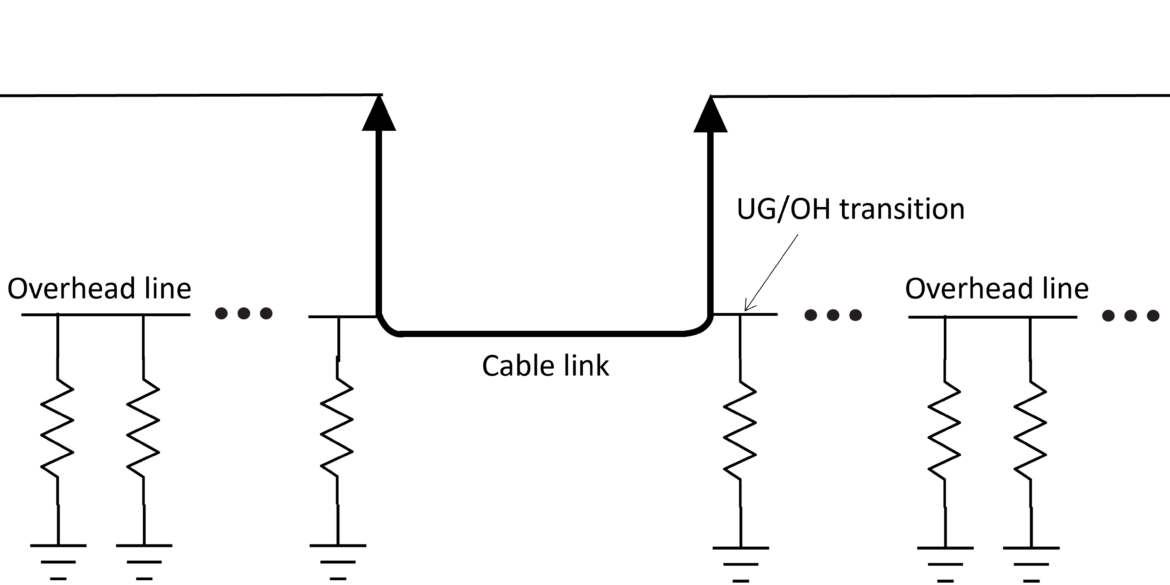
The second example system consists of an overhead transmission line connecting between two substations. Figure 3 depicts the system for this arrangement, in which the arrows indicate direction of current flows.
The flow of fault currents is described as follows:

If a single-phase to earth fault occurs, a portion of the total fault current will flow into the earthing system of Substation A as Grid Current (then back to the source) which gives rise to the touch and step voltage hazards. Another portion of the fault current will flow back via the overhead earth wire.
Since individual towers are earthed, there are also stray currents flowing to earth through the tower and their footings. To be more accurate, SafeGrid takes the effect of these stray currents into account when calculating the fault current distribution. Tower grid resistance and number of repeated subsections are thereby required.
Active conductors used in this example system are ACSR/AC Golf (54/3.00 mm, 431 mm2). Figure 4 shows an overhead lines arrangement at 110 kV voltage level. Earth wire used is SC/AC (7/3.75, 77.28 mm2).
The 110 kV transmission line is straight and a relatively short length of 10 km. The line consists of 21 tower structures which are the same along the length of the line (refer to Figure 4) and are each separated by a span length of 500 m.
Phase a is assumed to be the faulted phase as single phase to earth fault assumed.
")
Physical and electrical characteristics of overhead lines, earth wires and towers are shown in the Table 2.
Table 2 – Characteristics of overhead lines, earth wires and tower resistance
| Conductor diameter | Conductor AC resistance | Earth wire diameter | Earth wire AC resistance | Tower resistance |
|---|---|---|---|---|
| 27.0 mm | 0.0915 Ω/km | 11.3 mm | 1.463 Ω/km | 15 Ω |
Calculating the fault currents
The steps of using FCD module will be explained based on above two systems. Local singlephase to earth fault are considered as the fault type for both systems.

Select the standard case to match the installation.

According to the schematic diagram and cable bonding type, CASE 1 should be selected for example system A:
- Two Subs, Cables SC, Solid bonded, Local 1 ph-e fault
A schematic of the arrangement for this case as seen in SafeGrid is shown in Figure 6.
According to the schematic diagram and numbers of earth wire, CASE 13 should be selected
for example system B:
- Two Subs, Overhead, 1 earth wire, Local 1 ph-e fault
")
The standard case schematics can be described as follows:
The Nodes are where the voltages are calculated these are the numbered circles. The Elements are the lines connected between the nodes where current flows and are given a unique and descriptive name.

Enter data in all data inputs fields.
Depending on which standard case is selected will determine the data inputs which are displayed and needs to be entered.
See the following sections for a breakdown of what to enter for the two systems.
System A - Two substations connected by screened underground cables

Fault current is the total current which is 7 kA.
Length is 913 m which is the overall length between the two substations.
Soil electrical resistivity is assumed to be 100 Ω.m. Note a value which is representative of the actual soil resistivity should be used.
Earth grid (local) resistance is taken as the calculated value from within SafeGrid under Display Results. Figure 8 shows, the calculated grid resistance of the earthing grid system (not provided in this tutorial) is 2.077 Ω. Also refer to Figure 2, the resistance of WMTS earth grid is the local earth grid resistance.

Earth grid (remote) resistance is that of the remote substation to which the local earth grid is connected via terminating conductors and is nearest to the source of the fault current. Refer to Figure 2, the resistance of DA earth grid is the remote earth grid resistance.
Physical (relative) position of the conductors Cond. A-C positions, Y/Z must be entered in order to calculate the mutual impedances for coupled elements. These values are obtained from cable or overhead lines arrangements (refer to Figure 1 and Figure 4).
Phase cond. diameter and phase cond. a.c. resistance needs to be obtained from the Standards or manufacturer datasheets and entered in units Ω/km. Refer to Table 1, the AC resistance of phase conductor is 0.0388 Ω/km and the diameter is 29.9 mm.
Screen a.c. resistance, Screen outer diameter and Screen thickness can also be obtained from the Standards or manufacturer datasheets. Refer to Table 1, the screen diameter and thickness is 47.2 mm and 4.5 mm respectively, while screen AC resistance is 0.2893 Ω/km.
System B - Two substations connected by overhead transmission lines

Except for those same data inputs fields which are the same for system A, the inputs required for system B are explained below.
Length overall is the overall distance between two substations which is 10 km.
No. of subsections is determined by the overall length and span length between two towers. With an overall line length of 10 km the number of subsections is 20 since towers are separated by a span length of 500 m.
Cond. A position Z, Y are the physical position of the faulted phase which is located nearest to the earth wire (refer to Figure 4). In this case it is the phase conductor which is highest above ground level.
Earth A position Z, Y are the physical position of the earth wire (refer to Figure 4).
Earth outer diameter and earth a.c. resistance can be obtained from the manufacturer datasheet, which are 11.3 mm and 1.463 Ω/km respectively (refer to Table 2).
Tower resistance is 15 Ω (refer to Table 2). This is the average resistance of the individual tower earthing systems.
Results

Click Calculate to obtain the fault current distribution by nodal analysis.
The fault current results are shown at the right side of main window in SafeGrid.
The calculated fault current distribution results are shown as both a complex magnitude and as a percentage of the total of fault current for each unique conductive path (Element) in the system model.
Each element is given as ELEMENT NAME [start node no., end node no.]. The order of the start and end nodes helps determine the direction of the flow of fault currents based on the sign (+/-) of the magnitude.
The current flowing through EG LOCAL indicates the fault current that would be injected into the local substation earthing system.
Figure 10 shows for System A (screened cable connected) the fault current which flows into the EG LOCAL is 192 A which accounts for 3 % of total fault current.
Figure 11 shows for System B (overhead line connected) the fault current which flows into the local earth grid is 3857 A which accounts for 55 % of total fault current.
The reasons for the differences in results are explained below.
The separation between the faulted phase and earth return conductors affects the mutual impedance and hence the coupling with the fault current.
Due to the small physical separation between the faulted phase conductor of a cable system and the screens a very high proportion of the total fault current will return to the source via the screens rather than the local (faulted) earth system.
Still the proportion of the total fault current returning to the source via the earth wire for an overhead line connected system is also significant.
The calculated (reduced) fault current flowing into the local earthing system is then used as input for calculating the touch and step voltages for the substation.