The Magnetic Fields module in Cable HV Software calculates the magnetic field density in micro Tesla µT occurring around a cable, circuit or a group of circuits. The calculations are based on the Biot-Savart law which explains the fundamental quantitative relationship between an electric current which is flowing and the magnetic field it produces. The magnetic field produced by multiple conductors is calculated as the summation of the magnetic fields caused by the individual conductors.
Capabilities:
Cables in air or buried cables at any x, y position.
Any cable type (single core and multi-core) and any number of cables.
The current magnitude and direction of flow as well as phase angle can be changed.
Calculates magnetic field intensity at any height above the cables.
The effect of relative permeability
The following practical example will show you how to use the Magnetic Fields module.
A three-phase circuit example
A three-phase circuit without neutral is installed in a lava field. The parameters of the cable are shown in Table 1.
Table 1 – Cable data
Nominal section area (mm2)
Conductor diameter (mm)
DC conductor resistance (Ω/km)
Thickness of insulation
Aluminium screen
Lead sheath
Sectional area (mm2)
Outside diameter of cable
Sectional area (mm2)
Outside diameter of cable
2000 S1
57.2
0.0090
16.4
160
110
830
114
1 S: segmental stranded
Cables are directly buried at 0.8 m depth in flat arrangement (see Figure 1). The relative permeability of volcanic rock is assumed as 1.021. The thermal resistivity of volcanic rock is approximately 1.2 C.m/W.
Figure 1 – Installation of cables
The magnetic field density at ground level and 1 m above ground will be calculated for cable touching and for the following distances between cables (shown as d in Figure 1): 0.2m, 0.3m, 0.5m.
1. Obtain the current ratings
Based on the cable and installation conditions, the current rating can be calculated. The cable physical positions and steady-state current rating will then be imported to the Magnetic Fields module automatically.
Figure 2 – Obtain the current ratings
Edit and load the cable model by clicking Cable Models Hide/Show.
Alternatively, you can load a cable model from the library of pre-modelled power cables.
Select Buried of Installation method and specify relevant parameters to obtain a current rating or a set of current ratings for multiple cable circuits. In this case, arrangement of flat touching and flat spaced are set to obtain the current ratings.
Figure 3 – Cable installation and cable arrangement (flat touching)
The calculated current rating of flat touching is 1232 A. Adjusting the distance between cables, we can separately get current ratings for the distances of 0.2 m, 0.3 m, 0.5 m between cables. Their current ratings are shown in the Table 2.
Table 2 – Current rating of different arrangements
Arrangement
Flat-touching
Flat-spaced (0.2 m)
Flat-spaced (0.3m)
Flat-spaced (0.5m)
Current rating (A)
1232
1130
1044
963
The cable positions and steady-state current rating of flat-touching arrangement are automatically imported (Figure 4). After setting up every installation condition, the new cable positions and current rating will be imported every time you re-open the module.
Figure 4 – Cable positions and current ratings in Magnetic Fields module
2. Calculate the magnetic field density
The Magnetic Fields module calculates the magnetic field density at any height above the cables.
Figure 5 – Calculate the magnetic field intensity
Enter or edit the cable installation data by clicking the table cells. Click Add or Remove buttons to add or remove cables and click Reset to reset the table and remove all the data.
The cable installation data includes positions (note positive Y is buried depth), phase designation (A, B, C, L, N), current magnitude, phase angle, current direction or switch current On / Off.
Select Installation method and specify the Relative soil permeability of the Buried installation. The relative permeability of the in air installation is 1.
In this case, buried installation is selected and relative soil permeability is set as 1.021.
Specify the calculation parameters which provides the inputs for setting the plots.
The horizontal inputs determine how wide the sweep of values are for the magnetic field density plot(s). The vertical inputs determine the heights of the calculated plots above the ground surface (at 0 m) and the number of plots determined by the step size. Magnetic field density at ground level and at 1 m above ground level are calculated in this case.
Click Calculate to obtain the magnetic field intensity. The magnetic field intensity plots will then be calculated and updated. Calculate the magnetic field of other scenarios by editing the cable installation data or importing data from main application.
3. Make use of magnetic field intensity interactive plots
The plot displays the calculated magnetic field intensity results.
Move the cursor along the magnetic field intensity plots. Also click on the cables to display the physical positions.
Zoom or pan the plots by pressing corresponding buttons in the upper right corner.
Select or deselect plots to show or hide their magnetic field density results.
4. Create a report
Click Report to create a PDF report containing inputs and results of magnetic field density.
A snippet of the flat-touching arrangement report of is shown below.
Figure 7 – A snippet of the flat-touching arrangement report
The magnetic field density results of all arrangements are summarized in Table 3.
Figure 6 – Magnetic field density interactive plots
Table 3 – Maximum magnetic field density
Arrangement and calculated plots
Flat touching
Flat-spaced (0.2 m)
Flat-spaced (0.3 m)
Flat-spaced (0.5m)
Ground level
1 m above ground
Ground level
1 m above ground
Ground level
1 m above ground
Ground level
1 m above ground
Maximum
magnetic
field intensity
(µT)
75.54
15.12
117.50
24.16
153.62
33.07
201.33
48.91
The International Commission for the Protection against Non-Ionizing Radiation Protection Guide [2] has set 1 mT as the reference limit for occupational exposure and 200 μT as the public exposure limits [1-3]. In this case, the maximum magnetic field density at ground level of flat arrangement spaced by 0.5 m exceeds the public exposure limit.
References
[1] E. Fernandez and J. Patrick, “Magnetic Fields from High Voltage Power Cables,” 2018. [Online]. Available: https://elek.com/wp-content/uploads/2018/09/Magnetic-Fields-from-High-Voltage-Power-Cables.pdf. [2] M. Rüdiger et al., “(International Commission on Non-Ionizing Radiation Protection). ICNIRP Guidelines for Limiting Exposure to Electric Fields Induced by Movement of the Human Body in a Static Magnetic Field and by Time-Varying Magnetic Fields below 1 Hz,” 2014. [3] I. Guideline, “Guidelines for limiting exposure to time-varying electric, magnetic, and electromagnetic fields (up to 300 GHz),” Health phys, vol. 74, no. 4, pp. 494-522, 1998.
This video teaches the fundamentals of soil dry out and explains how it affects power cable ampacity calculations. Several example calculations are explained.
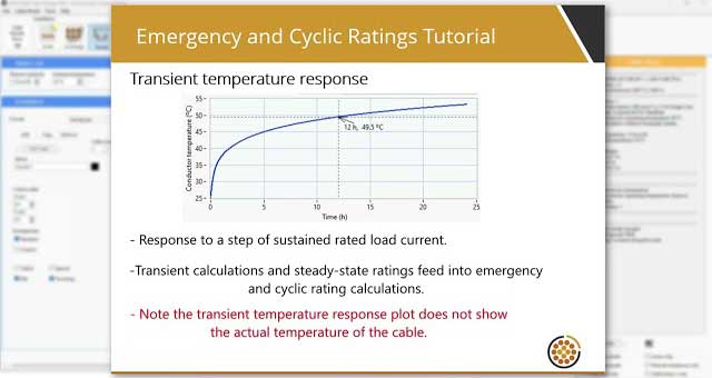
The Transient Rating module in ELEK Cable HV Software calculates the emergency and cyclic current rating of cables installed in air and buried cables, in accordance with IEC standards.
The Finite Element Method (FEM) module in ELEK Cable HV Software calculates the current rating of cables in custom arrangements and goes way beyond the limitations of the IEC Standards. For example, users can calculate the current rating for installations with multiple zones of different thermal resistivity.
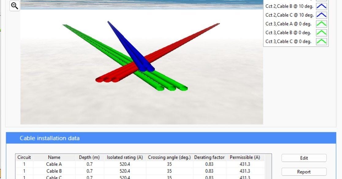
An example calculation of 132 kV single core and 22 kV three core cable circuits crossing where the derating factor for variation of the crossing angle is examined.


")